Together with Kyle Willett, one of the organizers of the Galaxy Challenge, I’ve written a paper about my winning solution for this competition. It is available on ArXiv.
The paper has been accepted for publication in MNRAS, a journal on astronomy and astrophysics, but is also aimed at people with a machine learning background. Due to this dual audience, it contains both an in-depth overview of deep learning and convolutional networks, and a thorough analysis of the resulting model and its potential impact for astronomy research.
There is some overlap with the blog post I wrote after the competition ended, but there is a lot more detail and background information, and the ‘results’ and ‘analysis’ sections are entirely new (although those of you who have seen one of my talks on the subject may have seen some of the images before).
I am very grateful to Kyle Willett for helping me write the manuscript. Without his help, writing a paper for an audience of astronomers would have been an impossible task for me. I believe it’s crucially important that applications of deep learning and machine learning in general get communicated to the people that could benefit from them, in such a way that they might actually consider using them.
I am also grateful to current and former supervisors, Joni Dambre and Benjamin Schrauwen, for supporting me when I was working on this competition and this paper, even though it is only tangentially related to the subject of my PhD.
The National Data Science Bowl, a data science competition where the goal was to classify images of plankton, has just ended. I participated with six other members of my research lab, the Reservoir lab of prof. Joni Dambre at Ghent University in Belgium. Our team finished 1st! In this post, we’ll explain our approach.
The ≋ Deep Sea ≋ team consisted of Aäron van den Oord, Ira Korshunova, Jeroen Burms, Jonas Degrave,
Lionel
Pigou, Pieter Buteneers and myself. We are all master students, PhD students and post-docs at Ghent University. We decided to participate together because we are all very interested in deep learning, and a collaborative effort to solve a practical problem is a great way to learn.
There were seven of us, so over the course of three months, we were able to try a plethora of different things, including a bunch of recently published techniques, and a couple of novelties. This blog post was written jointly by the team and will cover all the different ingredients that went into our solution in some detail.
This blog post is going to be pretty long! Here’s an overview of the different sections. If you want to skip ahead, just click the section title to go there.
The goal of the competition was to classify grayscale images of plankton into one of 121 classes. They were created using an underwater camera that is towed through an area. The resulting images are then used by scientists to determine which species occur in this area, and how common they are. There are typically a lot of these images, and they need to be annotated before any conclusions can be drawn. Automating this process as much as possible should save a lot of time!
The images obtained using the camera were already processed by a segmentation algorithm to identify and isolate individual organisms, and then cropped accordingly. Interestingly, the size of an organism in the resulting images is proportional to its actual size, and does not depend on the distance to the lens of the camera. This means that size carries useful information for the task of identifying the species. In practice it also means that all the images in the dataset have different sizes.
Participants were expected to build a model that produces a probability distribution across the 121 classes for each image. These predicted distributions were scored using the log loss (which corresponds to the negative log likelihood or equivalently the cross-entropy loss).
This loss function has some interesting properties: for one, it is extremely sensitive to overconfident predictions. If your model predicts a probability of 1 for a certain class, and it happens to be wrong, the loss becomes infinite. It is also differentiable, which means that models trained with gradient-based methods (such as neural networks) can optimize it directly - it is unnecessary to use a surrogate loss function.
Interestingly, optimizing the log loss is not quite the same as optimizing classification accuracy. Although the two are obviously correlated, we paid special attention to this because it was often the case that significant improvements to the log loss would barely affect the classification accuracy of the models.
The solution: convnets!
Image classification problems are often approached using convolutional neural networks these days, and with good reason: they achieve record-breaking performance on some really difficult tasks.
A challenge with this competition was the size of the dataset: about 30000 examples for 121 classes. Several classes had fewer than 20 examples in total. Deep learning approaches are often said to require enormous amounts of data to work well, but recently this notion has been challenged, and our results in this competition also indicate that this is not necessarily true. Judicious use of techniques to prevent overfitting such as dropout, weight decay, data augmentation, pre-training, pseudo-labeling and parameter sharing, has enabled us to train very large models with up to 27 million parameters on this dataset.
Some of you may remember that I participated in another Kaggle competition last year: the Galaxy Challenge. The goal of that competition was to classify images of galaxies. It turns out that a lot of the things I learned during that competition were also applicable here. Most importantly, just like images of galaxies, images of plankton are (mostly) rotation invariant. I used this property for data augmentation, and incorporated it into the model architecture.
Software and hardware
We used Python, NumPy and Theano to implement our solution, in combination with the cuDNN library. We also used PyCUDA to implement a few custom kernels.
Our code is mostly based on the Lasagne library, which provides a bunch of layer classes and some utilities that make it easier to build neural nets in Theano. This is currently being developed by a group of researchers with different affiliations, including Aäron and myself. We hope to release the first version soon!
We also used scikit-image for pre-processing and augmentation, and ghalton for quasi-random number generation. During the competition, we kept track of all of our results in a Google Drive spreadsheet. Our code was hosted on a private GitHub repository, with everyone in charge of their own branch.
We trained our models on the NVIDIA GPUs that we have in the lab, which include GTX 980, GTX 680 and Tesla K40 cards.
We performed very little pre-processing, other than rescaling the images in various ways and then performing global zero mean unit variance (ZMUV) normalization, to improve the stability of training and increase the convergence speed.
Rescaling the images was necessary because they vary in size a lot: the smallest ones are less than 40 by 40 pixels, whereas the largest ones are up to 400 by 400 pixels. We experimented with various (combinations of) rescaling strategies. For most networks, we simply rescaled the largest side of each image to a fixed length.
We also tried estimating the size of the creatures using image moments. Unfortunately, centering and rescaling the images based on image moments did not improve results, but they turned out to be useful as additional features for classification (see below).
Data augmentation
We augmented the data to artificially increase the size of the dataset. We used various affine transforms, and gradually increased the intensity of the augmentation as our models started to overfit more. We ended up with some pretty extreme augmentation parameters:
rotation: random with angle between 0° and 360° (uniform)
translation: random with shift between -10 and 10 pixels (uniform)
rescaling: random with scale factor between 1/1.6 and 1.6 (log-uniform)
flipping: yes or no (bernoulli)
shearing: random with angle between -20° and 20° (uniform)
stretching: random with stretch factor between 1/1.3 and 1.3 (log-uniform)
We augmented the data on-demand during training (realtime augmentation), which allowed us to combine the image rescaling and augmentation into a single affine transform. The augmentation was all done on the CPU while the GPU was training on the previous chunk of data.
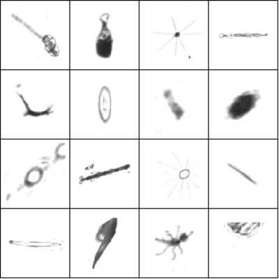
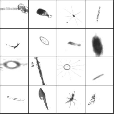
Pre-processed images (left) and augmented versions of the same images (right).
We experimented with elastic distortions at some point, but this did not improve performance although it reduced overfitting slightly. We also tried sampling the augmentation transform parameters from gaussian instead of uniform distributions, but this did not improve results either.
Most of our convnet architectures were strongly inspired by OxfordNet: they consist of lots of convolutional layers with 3x3 filters. We used ‘same’ convolutions (i.e. the output feature maps are the same size as the input feature maps) and overlapping pooling with window size 3 and stride 2.
We started with a fairly shallow models by modern standards (~ 6 layers) and gradually added more layers when we noticed it improved performance (it usually did). Near the end of the competition, we were training models with up to 16 layers. The challenge, as always, was balancing improved performance with increased overfitting.
We experimented with strided convolutions with 7x7 filters in the first two layers for a while, inspired by the work of He et al., but we were unable to achieve the same performance with this in our networks.
Cyclic pooling
When I participated in the Galaxy Challenge, one of the things I did differently from other competitors was to exploit the rotational symmetry of the images to share parameters in the network. I applied the same stack of convolutional layers to several rotated and flipped versions of the same input image, concatenated the resulting feature representations, and fed those into a stack of dense layers. This allowed the network to use the same feature extraction pipeline to “look at” the input from different angles.
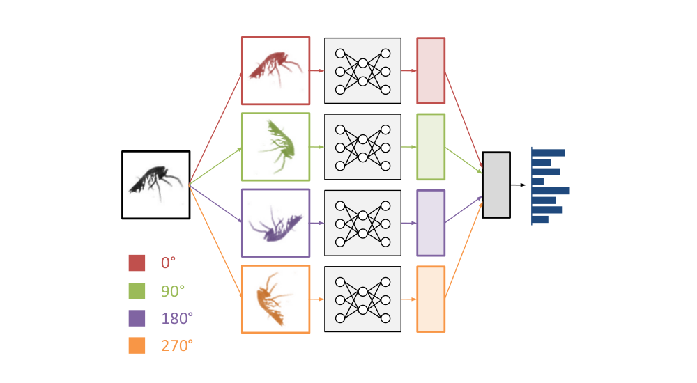
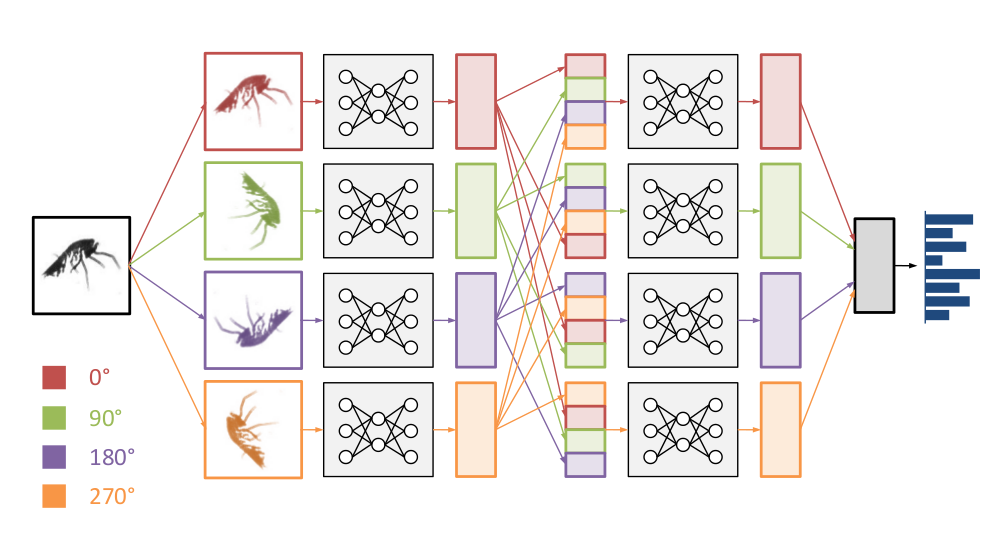
Here, we took this a step further. Rather than concatenating the feature representations, we decided to pool across them to get rotation invariance. Here’s how it worked in practice: the images in a minibatch occur 4 times, in 4 different orientations. They are processed by the network in parallel, and at the top, the feature maps are pooled together. We decided to call this cyclic pooling, after cyclic groups.
Schematic representation of a convnet with cyclic pooling.
The nice thing about 4-way cyclic pooling is that it can be implemented very efficiently: the images are rotated by 0, 90, 180 and 270 degrees. All of these rotations can be achieved simply by transposing and flipping image axes. That means no interpolation is required.
Cyclic pooling also allowed us to reduce the batch size by a factor of 4: instead of having batches of 128 images, each batch now contained 32 images and was then turned into a batch with an effective size of 128 again inside the network, by stacking the original batch in 4 orientations. After the pooling step, the batch size was reduced to 32 again.
We tried several pooling functions over the course of the competition, as well as different positions in the network for the pooling operation (just before the output layer, between hidden layers, …). It turned out that root-mean-square pooling gave much better results than mean pooling or max pooling. We weren’t able to find a good explanation for this, but we suspect it may have something to do with rotational phase invariance.
One of our models pooled over 8 rotations, spaced apart 45 degrees. This required generating the input images at two angles (0 and 45 degrees). We also considered having the model do 8-way pooling by including flipped versions of each rotated image copy (dihedral pooling, after dihedral groups). Unfortunately this did not work better.
‘Rolling’ feature maps
Cyclic pooling modestly improved our results, but it can be taken a step further. A cyclic pooling convnet extracts features from input images in four different orientations. An alternative interpretation is that its filters are applied to the input images in four different orientations. That means we can combine the stacks of feature maps from the different orientations into one big stack, and then learn the next layer of features on this combined input. As a result, the network then appears to have 4 times more filters than it actually has!
This is cheap to do, since the feature maps are already being computed anyway. We just have to combine them together in the right order and orientation. We named the operation that combines feature maps from different orientations a roll.
Schematic representation of a roll operation inside a convnet with cyclic pooling.
Roll operations can be inserted after dense layers or after convolutional layers. In the latter case, care has to be taken to rotate the feature maps appropriately, so that they are all aligned.
We originally implemented the operations with a few lines of Theano code. This is a nice demonstration of Theano’s effectiveness for rapid prototyping of new ideas. Later on we spent some time implementing CUDA kernels for the roll operations and their gradients, because networks with many rolled layers were getting pretty slow to train. Using your own CUDA kernels with Theano turns out to be relatively easy in combination with PyCUDA. No additional C-code is required.
In most of the models we evaluated, we only inserted convolutional roll operations after the pooling layers, because this reduced the size of the feature maps that needed to be copied and stacked together.
Note that it is perfectly possible to build a cyclic pooling convnet without any roll operations, but it’s not possible to have roll operations in a network without cyclic pooling. The roll operation is only made possible because the cyclic pooling requires that each input image is processed in four different orientations to begin with.
Nonlinearities
We experimented with various variants of rectified linear units (ReLUs), as well as maxout units (only in the dense layers). We also tried out smooth non-linearities and the ‘parameterized ReLUs’ that were recently introduced by He et al., but found networks with these units to be very prone to overfitting.
However, we had great success with (very) leaky ReLUs. Instead of taking the maximum of the input and zero, y = max(x, 0), leaky ReLUs take the maximum of the input and a scaled version of the input, y = max(x, a*x). Here, a is a tunable scale parameter. Setting it to zero yields regular ReLUs, and making it trainable yields parameterized ReLUs.
For fairly deep networks (10+ layers), we found that varying this parameter between 0 and 1/2 did not really affect the predictive performance. However, larger values in this range significantly reduced the level of overfitting. This in turn allowed us to scale up our models further. We eventually settled on a = 1/3.
Spatial pooling
We started out using networks with 2 or 3 spatial pooling layers, and we initially had some trouble getting networks with more pooling stages to work well. Most of our final models have 4 pooling stages though.
We started out with the traditional approach of 2x2 max-pooling, but eventually switched to 3x3 max-pooling with stride 2 (which we’ll refer to as 3x3s2), mainly because it allowed us to use a larger input size while keeping the same feature map size at the topmost convolutional layer, and without increasing the computational cost significantly.
As an example, a network with 80x80 input and 4 2x2 pooling stages will have feature maps of size 5x5 at the topmost convolutional layer. If we use 3x3s2 pooling instead, we can feed 95x95 input and get feature maps with the same 5x5 shape. This improved performance and only slowed down training slightly.
Multiscale architectures
As mentioned before, the images vary widely in size, so we usually rescaled them using the largest dimension of the image as a size estimate. This is clearly suboptimal, because some species of plankton are larger than others. Size carries valuable information.
To allow the network to learn this, we experimented with combinations of different rescaling strategies within the same network, by combining multiple networks with different rescaled inputs together into ‘multiscale’ networks.
What worked best was to combine a network with inputs rescaled based on image size, and a smaller network with inputs rescaled by a fixed factor. Of course this slowed down training quite a bit, but it allowed us to squeeze out a bit more performance.
Additional image features
We experimented with training small neural nets on extracted image features to ‘correct’ the predictions of our convnets. We referred to this as ‘late fusing’ because the feature network and the convnet were joined only at the output layer (before the softmax). We also tried joining them at earlier layers, but consistently found this to work worse, because of overfitting.
We thought this could be useful, because the features can be extracted from the raw (i.e. non-rescaled) images, so this procedure could provide additional information that is missed by the convnets. Here are some examples of types of features we evaluated (the ones we ended up using are in bold):
Image size in pixels
Size and shape estimates based on image moments
Hu moments
Zernike moments
Parameter Free Threshold Adjacency Statistics
Linear Binary Patterns
Haralick texture features
Features from the competition tutorial
Combinations of the above
The image size, the features based on image moments and the Haralick texture features were the ones that stood out the most in terms of performance. The features were fed to a neural net with two dense layers of 80 units. The final layer of the model was fused with previously generated predictions of our best convnet-based models. Using this approach, we didn’t have to retrain the convnets nor did we have to regenerate predictions (which saved us a lot of time).
To deal with variance due to the random weight initialization, we trained each feature network 10 times and blended the copies with uniform weights. This resulted in a consistent validation loss decrease of 0.01 (or 1.81%) on average, which was quite significant near the end of the competition.
Interestingly, late fusion with image size and features based on image moments seems to help just as much for multiscale models as for regular convnets. This is a bit counterintuitive: we expected both approaches to help because they could extract information about the size of the creatures, so the obtained performance improvements would overlap. The fact they were fully orthogonal was a nice surprise.
Example convnet architecture
Here’s an example of an architecture that works well. It has 13 layers with parameters (10 convolutional, 3 fully connected) and 4 spatial pooling layers. The input shape is (32, 1, 95, 95), in bc01 order (batch size, number of channels, height, width). The output shape is (32, 121). For a given input, the network outputs 121 probabilities that sum to 1, one for each class.
Layer type
Size
Output shape
cyclic slice
(128, 1, 95, 95)
convolution
32 3x3 filters
(128, 32, 95, 95)
convolution
16 3x3 filters
(128, 16, 95, 95)
max pooling
3x3, stride 2
(128, 16, 47, 47)
cyclic roll
(128, 64, 47, 47)
convolution
64 3x3 filters
(128, 64, 47, 47)
convolution
32 3x3 filters
(128, 32, 47, 47)
max pooling
3x3, stride 2
(128, 32, 23, 23)
cyclic roll
(128, 128, 23, 23)
convolution
128 3x3 filters
(128, 128, 23, 23)
convolution
128 3x3 filters
(128, 128, 23, 23)
convolution
64 3x3 filters
(128, 64, 23, 23)
max pooling
3x3, stride 2
(128, 64, 11, 11)
cyclic roll
(128, 256, 11, 11)
convolution
256 3x3 filters
(128, 256, 11, 11)
convolution
256 3x3 filters
(128, 256, 11, 11)
convolution
128 3x3 filters
(128, 128, 11, 11)
max pooling
3x3, stride 2
(128, 128, 5, 5)
cyclic roll
(128, 512, 5, 5)
fully connected
512 2-piece maxout units
(128, 512)
cyclic pooling (rms)
(32, 512)
fully connected
512 2-piece maxout units
(32, 512)
fully connected
121-way softmax
(32, 121)
Note how the ‘cyclic slice’ layer increases the batch size fourfold. The ‘cyclic pooling’ layer reduces it back to 32 again near the end. The ‘cyclic roll’ layers increase the number of feature maps fourfold.
We split off 10% of the labeled data as a validation set using stratified sampling. Due to the small size of this set, our validation estimates were relatively noisy and we periodically validated some models on the leaderboard as well.
Training algorithm
We trained all of our models with stochastic gradient descent (SGD) with Nesterov momentum. We set the momentum parameter to 0.9 and did not tune it further. Most models took between 24 and 48 hours to train to convergence.
We trained most of the models with about 215000 gradient steps and eventually settled on a discrete learning rate schedule with two 10-fold decreases (following Krizhevsky et al.), after about 180000 and 205000 gradient steps respectively. For most models we used an initial learning rate of 0.003.
We briefly experimented with the Adam update rule proposed by Kingma and Ba, as an alternative to Nesterov momentum. We used the version of the algorithm described in the first version of the paper, without the lambda parameter. Although this seemed to speed up convergence by a factor of almost 2x, the results were always slightly worse than those achieved with Nesterov momentum, so we eventually abandoned this idea.
Initialization
We used a variant of the orthogonal initialization strategy proposed by Saxe et al. everywhere. This allowed us to add as many layers as we wanted without running into any convergence problems.
Regularization
For most models, we used dropout in the fully connected layers of the network, with a dropout probability of 0.5. We experimented with dropout in the convolutional layers as well for some models.
We also tried Gaussian dropout (using multiplicative Gaussian noise instead of multiplicative Bernoulli noise) and found this to work about as well as traditional dropout.
We discovered near the end of the competition that it was useful to have a small amount of weight decay to stabilize training of larger models (so not just for its regularizing effect). Models with large fully connected layers and without weight decay would often diverge unless the learning rate was decreased considerably, which slowed things down too much.
Since the test set was much larger than the training set, we experimented with using unsupervised pre-training on the test set to initialize the networks. We only pre-trained the convolutional layers, using convolutional auto-encoders (CAE, Masci. et al.). This approach consists of building a stack of layers implementing the reverse operations (i.e. deconvolution and unpooling) of the layers that are to be pre-trained. These can then be used to try and reconstruct the input of those layers.
In line with the literature, we found that pre-training a network serves as an excellent regularizer (much higher train error, slightly better validation score), but the validation results with test-time augmentation (see below) were consistently slightly worse for some reason.
Pre-training might allow us to scale our models up further, but because they already took a long time to train, and because the pre-training itself was time-consuming as well, we did not end up doing this for any of our final models.
To learn useful features with unsupervised pre-training, we relied on the max-pooling and unpooling layers to serve as a sparsification of the features. We did not try a denoising autoencoder approach for two reasons: first of all, according to the results described by Masci et al., the max- and unpooling approach produces way better filters than the denoising approach, and the further improvement of combining these approaches is negligible. Secondly, due to how the networks were implemented, it would slow things down a lot.
We tried different setups for this pre-training stage:
greedy layerwise training vs. training the full deconvolutional stack jointly: we obtained the best results when pre-training the full stack jointly. Sometimes it was necessary to initialize this stack using the greedy approach to get it to work.
using tied weights vs. using untied weights: Having the weights in the deconvolutional layers be the transpose of those in the corresponding convolutional layers made the (full) autoencoder easier and much faster to train. Because of this, we never got the CAE with untied weights to reconstruct the data as well as the CAE with tied weights, despite having more trainable parameters.
We also tried different approaches for the supervised finetuning stage. We observed that without some modifications to our supervised training setup, there was no difference in performance between a pre-trained network and a randomly initialized one. Possibly, by the time the randomly initialized dense layers are in a suitable parameter range, the network has already forgotten a substantial amount of the information it acquired during the pre-training phase.
We found two ways to overcome this:
keeping the pre-trained layers fixed for a while: before training the full networks, we only train the (randomly initialized) dense layers. This is quite fast since we only need to backpropagate through the top few layers. The idea is that we put the network more firmly in the basin of attraction the pre-training led us to.
Halving the learning rate in the convolutional layers: By having the dense layers adapt faster to the (pre-trained) convolutional layers, the network is less likely to make large changes to the pre-trained parameters before the dense layers are in a good parameter range.
Both approaches produced similar results.
Pseudo-labeling
Another way we exploited the information in the test set was by a combination of pseudo-labeling and knowledge distillation (Hinton et al.). The initial results from models trained with pseudo-labeling were significantly better than we anticipated, so we ended up investigating this approach quite thoroughly.
Pseudo-labeling entails adding test data to the training set to create a much larger dataset. The labels of the test datapoints (so called pseudo-labels) are based on predictions from a previously trained model or an ensemble of models. This mostly had a regularizing effect, which allowed us to train bigger networks.
We experimented both with hard targets (one-hot coded) and soft targets (predicted probabilities), but quickly settled on soft targets as these gave much better results.
Another important detail is the balance between original data and pseudo-labeled data in the resulting dataset. In most of our experiments 33% of the minibatch was sampled from the pseudolabeled dataset and 67% from the real training set.
It is also possible to use more pseudo-labeled data points (e.g. 67%). In this case the model is regularized a lot more, but the results will be more similar to the pseudolabels. As mentioned before, this allowed us to train bigger networks, but in fact this is necessary to make pseudo-labeling work well. When using 67% of the pseudo-labeled dataset we even had to reduce or disable dropout, or the models would underfit.
Our pseudo-labeling approach differs from knowledge distillation in the sense that we use the test set instead of the training set to transfer knowledge between models. Another notable difference is that knowledge distillation is mainly intended for training smaller and faster networks that work nearly as well as bigger models, whereas we used it to train bigger models that perform better than the original model(s).
We think pseudo-labeling helped to improve our results because of the large test set and the combination of data-augmentation and test-time augmentation (see below). When pseudo-labeled test data is added to the training set, the network is optimized (or constrained) to generate predictions similar to the pseudo-labels for all possible variations and transformations of the data resulting from augmentation. This makes the network more invariant to these transformations, and forces the network to make more meaningful predictions.
We saw the biggest gains in the beginning (up to 0.015 improvement on the leaderboard), but even in the end we were able to improve on very large ensembles of (bagged) models (between 0.003 - 0.009).
We combined several forms of model averaging in our final submissions.
Test-time augmentation
For each individual model, we computed predictions across various augmented versions of the input images and averaged them. This improved performance by quite a large margin. When we started doing this, our leaderboard score dropped from 0.7875 to 0.7081. We used the acronym TTA to refer to this operation.
Initially, we used a manually created set of affine transformations which were applied to each image to augment it. This worked better than using a set of transformations with randomly sampled parameters. After a while, we looked for better ways to tile the augmentation parameter space, and settled on a quasi-random set of 70 transformations, using slightly more modest augmentation parameter ranges than those used for training.
Computing model predictions for the test set using TTA could take up to 12 hours, depending on the model.
Finding the optimal transformation instead of averaging
Since the TTA procedure improved the score considerably, we considered the possibility of optimizing the augmentation parameters at prediction time. This is possible because affine transformations are differentiable with respect to their parameters.
In order to do so, we implemented affine transformations as layers in a network, so that we could backpropagate through them. After the transformation is applied to an image, a pixel can land in between two positions of the pixel grid, which makes interpolation necessary. This makes finding these derivatives quite complex.
We tried various approaches to find the optimal augmentation, including the following:
Optimizing the transformation parameters to maximize (or minimize) the confidence of the predictions.
Training a convnet to predict the optimal transformation parameters for another convnet to use.
Unfortunately we were not able to improve our results with any of these approaches. This may be because selecting an optimal input augmentation as opposed to averaging across augmentations removes the regularizing effect of the averaging operation. As a consequence we did not use this technique in our final submissions, but we plan to explore this idea further.
Animated visualization of the optimization of the affine transformation parameters.
Combining different models
In total we trained over 300 models, so we had to select how many and which models to use in the final blend. For this, we used cross-validation on our validation set. On each fold, we optimized the weights of all models to minimize the loss of the ensemble on the training part.
We regularly created new ensembles from a different number of top-weighted models, which we further evaluated on the testing part. In the end, this could give an approximate idea of suitable models for ensembling.
Once the models were selected, they were blended uniformly or with weights optimized on the validation set. Both approaches gave comparable results.
The models selected by this process were not necessarily the ones with the lowest TTA score. Some models with relatively poor scores were selected because they make very different predictions than our other models. A few models had poor scores due to overfitting, but were selected nevertheless because the averaging reduces the effect of overfitting.
Bagging
To improve the score of the ensemble further, we replaced some of the models by an average of 5 models (including the original one), where each model was trained on a different subset of the data.
Here are a few other things we tried, with varying levels of success:
untied biases: having separate biases for each spatial location in the convolutional layer seemed to improve results very slightly.
winner take all nonlinearity (WTA, also known as channel-out) in the fully connected layers instead of ReLUs / maxout.
smooth nonlinearities: to increase the amount of variance in our blends we tried replacing the leaky rectified linear units with a smoothed version. Unfortunately this worsened our public leaderboard score.
specialist models: we tried training special models for highly confusable classes of chaetognaths, some protists, etc. using the knowledge distillation approach described by Hinton et al.. We also tried a self-informed neural network structure learning (Warde-Farley et al.), but in both cases the improvements were negligible.
batch normalization: unfortunately we were unable to reproduce the spectacular improvements in convergence speed described by Ioffe and Szegedy for our models.
Using FaMe regularization as described by Rudy et al. instead of dropout increased overfitting a lot. The regularizing effect seemed to be considerably weaker.
Semi-supervised learning with soft and hard bootstrapping as described by Reed et al. did not improve performance or reduce overfitting.
Here’s a non-exhaustive list of things that we found to reduce overfitting (including the obvious ones):
dropout (various forms)
aggressive data augmentation
suitable model architectures (depth and width of the layers influence overfitting in complicated ways)
weight decay
unsupervised pre-training
cyclic pooling (especially with root-mean-square pooling)
leaky ReLUs
pseudo-labeling
We also monitored the classification accuracy of our models during the competition. Our best models achieved an accuracy of over 82% on the validation set, and a top-5 accuracy of over 98%. This makes
it possible to use the model as a tool for speeding up manual annotation.
We had a lot of fun working on this problem together and learned a lot! If this problem interests you, be sure to check out the competition forum. Many of the participants will be posting overviews of their approaches in the coming days.
Congratulations to the other winners, and our thanks to the competition organizers and sponsors. We would also like to thank our supervisor Joni Dambre for letting us work on this problem together.
We will clean up our code and put it on GitHub soon. If you have any questions or feedback about this post, feel free to leave a comment.
One of our team, Ira Korshunova, is currently looking for a good research lab to start her PhD next semester. She can be contacted at irene.korshunova@gmail.com.
Guest post:Jan Schlüter from the OFAI, a fellow MIR researcher I have met at several conferences, recently added a feature to Theano that fits so well with my previoustwo posts on fast convolutions that we decided to include his writeup on my blog. So enjoy the third part of the series, written by Jan!
Over the past year, Theano has accumulated several alternative implementations for 2D convolution, the most costly operation in Convolutional Neural Networks.
There is no single implementation that is the fastest for all possible image and kernel shapes,
but with Theano you can mix and match them at will.
Now mixing and matching is something that can be easily automated: Meet meta-optimization!
The idea is to automatically select the fastest available implementation for each individual convolution operation in a Theano function, simply by timing them.
The feature is already available in Theano: If you install the latest version from github, you can activate it by setting the environment variable THEANO_FLAGS=optimizer_including=conv_meta,metaopt.verbose=1.
In the following, I will explain what it does, how it works, and demonstrate that it can outperform all existing convnet libraries.
Batched convolution
Before we begin, note that the convolution operation in Convolutional Neural Networks (CNNs) as used for Computer Vision is not just a convolution of a single 2D input image with a single 2D filter kernel.
For one, the input image can have multiple channels, such as a color image composed of three values per pixel. It can thus be expressed as a 3D tensor. To match this, the filter kernel has as many values per pixel as the input image, which makes it a 3D tensor as well. When computing the output, each channel is convolved separately with its corresponding kernel, and the resulting images are added up to produce a single 2D output image.
But usually, each convolutional layer returns a multi-channel output (a 3D tensor), which is achieved by learning multiple sets of kernels (a 4D tensor).
Finally, images are often propagated through the network in mini-batches of maybe 64 or 256 items to be processed independently, so the input and output become 4D tensors.
Putting everything together, the batched convolution operation convolves a 4D input tensor with a 4D kernel tensor to produce a 4D output tensor. Obviously, this gives ample of opportunities for parallelization. Add to this the different possible ways of computing a 2D convolution, and you can see why there are so many competing implementations.
The repertoire
As an actively maintained open-source project with several external contributors, Theano has grown to have access to five convolution implementations:
a “legacy” implementation that has been created for Theano
Nvidia’s new cuDNN library, via a wrapper done by Arnaud and subsequently improved by Frédéric and me
All of these have their strengths and weaknesses.
cuda-convnet only supports square kernels and places several restrictions on the number of input and output channels and the batch size.
The FFT-based based convolution is applicable to any configuration, but requires a lot of extra memory that practically limits it to small batch and image sizes or very potent graphics cards.
cuDNN requires a GPU of Compute Capability 3.0 or above,
and the convolution ported from Caffe needs some extra memory again.
Finally, the legacy implementation comes free of limitations, but is usually the slowest of the pack.
Depending on the configuration – that is, the batch size, image shape, filter count and kernel shape –, any of these five implementations can be the fastest.
Three convolutions per layer
To complicate matters, each convolutional layer in a convnet actually results in three batched convolution operations to be performed in training:
The forward pass, a valid convolution of images and kernels
The gradient wrt. weights, a valid convolution of images and the gradient wrt. output
The gradient wrt. input, a full convolution of the kernels and the gradient wrt. output
For a valid convolution, the kernel is applied wherever it completely overlaps with the input (i.e., it only touches valid data).
For a full convolution, it is applied wherever it overlaps with the input by at least one pixel –
this is equivalent to padding the input with a suitably-sized symmetric border of zeros and applying a valid convolution.
(For the eager ones: The third one in the list above is actually a correlation, because the kernels are not flipped as in the forward pass. And the second one requires the batch size and channels of the input, kernel and output tensors to be swapped. Still all of these can be expressed using the batched convolution operation described in the beginning.)
The “big libraries” (cuda-convnet, Caffe and cuDNN) each come with three algorithms specialized for these three cases, while the FFT-based convolution just distinguishes between valid and full convolutions.
Cherry-picking
A lot of my work on Theano’s convolution was triggered by following Soumith Chintala’s convnet-benchmarks initiative, which set out to compare all freely available Convolutional Neural Network libraries in terms of their performance.
When looking at some of the first results posted, the first thing I noticed was that it would pay off to use a different library for each of the five configurations tested. This has quickly been included as a hypothetical “cherry-picking” row into the result tables.
I took over maintenance of Soumith’s Theano benchmark script and evolved it into a handy little tool to compare its convolution implementations for different configurations. Feel free to download the script and follow along.
So let’s see what we could gain with cherry-picking in Theano:
What we see here are the respective computation times in milliseconds for a particular configuration (tensor shapes) for the legacy implementation, FFT-based convolution, cuDNN, gemm-based convolution and cuda-convnet (with two different values for a tuning parameter).
For this layer, cuDNN would be the optimal choice.
This time, the FFT-based convolution is faster, but the truly optimal choice would be combining it with cuda-convnet.
We see that the meta-optimizer should not just cherry-pick a different implementation per convolutional layer, but even a different implementation for each of the three convolutions in a layer – something that was not possible in Theano before (nor in any other library I am aware of).
The “swapping trick”
As you recall, cuda-convnet, Caffe and cuDNN come with specialized algorithms for the three convolutions per layer.
Interestingly, when porting the gemm-based convolution from Caffe to Theano, I noticed that the effort I put in properly using its two backward pass algorithms when applicable did not always pay off: For some configurations, it was faster to just use the forward pass algorithm instead, transposing tensors as needed.
I thus added a shape-based heuristic to select the fastest algorithm for the gemm-based convolution (making Theano’s port faster than Caffe for some configurations).
When adding support for Nvidia’s cuDNN library, Arnaud understandably assumed that it would hide this complexity from the user and select the optimal algorithm internally. So at first, Theano did not tell cuDNN whether a particular convolution’s purpose was a forward pass or one of the backward passes. When I changed the implementation accordingly, I again noticed that while performance generally improved a lot, for some configurations, using the “wrong” algorithm was actually faster.
Just as for Caffe, we can use this knowledge to be faster than cuDNN.
As the implementation is unknown, we cannot easily define a heuristic for choosing between the cuDNN algorithms.
However, the meta-optimizer can just try all applicable algorithms and see which one is the fastest.
I found it to suffice to just try two algorithms per convolution:
For the forward pass, try the “correct” algorithm and the gradient wrt. weights (both are valid convolutions)
For the gradient wrt. weights, try the “correct” algorithm and the forward pass
For the gradient wrt. inputs, try the “correct” algorithm and the forward pass (with additional zero padding to make it a full convolution)
I call this the “swapping trick” because it often leads to the first two algorithms being swapped.
Implementation
To understand why Theano was a perfect fit to add automatic algorithm selection, we will need to explain a bit of its inner workings.
First, Theano is not a neural network library, but a mathematical expression compiler.
In contrast to, say, Caffe, its basic components are not neural network layers, but mathematical operations.
Implementing a neural network is done by composing the expression for the forward pass (which will probably include matrix multiplications, vector additions, elementwise nonlinearities and possibly batched convolution and pooling), using this to build an expression for the training cost, and then letting Theano transform it into expressions for the gradients wrt. the parameters to be learned.
Finally, the expressions are compiled into functions that evaluate them for specific settings of the free variables (such as a mini-batch of training data).
But right before an expression is compiled, it is optimized, and this is where all the magic happens.
The expression is represented as a graph of Apply nodes (operations) and Variable nodes (the inputs and outputs of an operation), and Theano comes with a bunch of graph optimizers that modify the graph to produce the same result either more efficiently or more numerically stable.
One particular graph optimizer moves convolution operations from the CPU to the GPU by replacing the respective Apply node and adding the necessary transfer operations around it.
A whole set of graph optimizers then replaces the legacy GPU convolution operation with one of the more efficient implementations available in Theano. These optimizers have relative priorities and can be enabled and disabled by the user.
The new meta-optimizer is just another graph optimizer with a twist: When it encounters a convolution operation, it applies each of the set of available graph optimizers (plus the cuDNN “swapping trick” optimizer) in sequence, each time compiling and executing the subgraph performing the convolution, and chooses the one resulting in the best performance.
(Finally, this explains why it’s called meta-optimization.)
As the basic components in Theano are the mathematical operations, there is no extra work needed to be able to choose different implementations for the three convolutions per layer: All Theano sees when optimizing and compiling an expression is a graph containing several anonymous convolution operations, so it will naturally optimize each of them separately.
Practical gains
Let us now put the meta-optimizer to test using the benchmark script mentioned in the cherry-picking section:
In verbose mode, the meta-optimizer reports which implementations are tested, how each of them performs and which one is finally chosen.
For the configuration at hands, it turns out that the FFT-based implementation is fastest for the forward pass and the gradient wrt. weights, and cuDNN is fastest for the gradient wrt. inputs – but only when using the “wrong” algorithm for it (namely, cuDNN’s forward pass algorithm with zero padding, tried according to the swapping trick).
In all three instances, the optimal algorithm is about twice as fast as just choosing cuDNN, which would have been Theano’s current default behavior.
When training a full network, the impact will generally be smaller, because the convolution operations only constitute a part of the expressions evaluated (but often the most costly part).
The improvement also heavily depends on the input and kernel shapes – for a wide range of configurations, just using cuDNN for all convolutions is nearly optimal.
Still, a colleague of Sander reported a threefold performance improvement for a network trained for a Kaggle competition, with the meta-optimizer combining FFT, Caffe, and cuDNN with and without the swapping trick.
To get an estimate on how much Theano could help for your use case, just run the benchmark script for the configurations occurring in a forward pass through your network.
If you already use Theano, just set THEANO_FLAGS=optimizer_including=conv_meta to rest assured you will always make the most out of the time (and electricity!) you spend on training your networks.
Future
While the basic machinery is in place and works fine, there are a lot of conceivable improvements:
The meta-optimizer should cache its results on disk to speed up repeated compilations of the same graph.
Right now, the meta-optimizer uses all available convolution operations in Theano; it should be possible to control this.
As cuda-convnet is not included in Theano, but an external project (Pylearn2), it is not included in the meta-optimizer. However, it is possible to register additional optimizers at runtime via theano.sandbox.cuda.opt.conv_metaopt.register(). It would be nice to write such a pluggable optimizer for cuda-convnet.
Similarly, it would be nice to have a wrapper for cuda-convnet2 (in a separate repository) along with an optimizer to be registered with the meta-optimizer.
Currently, meta-optimization can only be used for non-strided valid or full convolutions, because this is what the legacy implementation is limited to. Changing this would require some refactoring, but lead to cleaner code and slightly improved performance.
Finally, it could be worthwhile to repeat the same for the pooling operation of CNNs: Port additional implementations to Theano, benchmark them and add a meta-optimizer.
Watch Issue #2072 on github for any progress on this, or even better, step in and implement one of these features if you can use it!
Both that issue and theano-dev are well-suited to ask for hints about implementing any of these TODOs – we’d be glad to have you on board.
This summer, I’m interning at Spotify in New York City, where I’m working on content-based music recommendation using convolutional neural networks. In this post, I’ll explain my approach and show some preliminary results.
Overview
This is going to be a long post, so here’s an overview of the different sections. If you want to skip ahead, just click the section title to go there.
Traditionally, Spotify has relied mostly on collaborative filtering approaches to power their recommendations. The idea of collaborative filtering is to determine the users’ preferences from historical usage data. For example, if two users listen to largely the same set of songs, their tastes are probably similar. Conversely, if two songs are listened to by the same group of users, they probably sound similar. This kind of information can be exploited to make recommendations.
Pure collaborative filtering approaches do not use any kind of information about the items that are being recommended, except for the consumption patterns associated with them: they are content-agnostic. This makes these approaches widely applicable: the same type of model can be used to recommend books, movies or music, for example.
Unfortunately, this also turns out to be their biggest flaw. Because of their reliance on usage data, popular items will be much easier to recommend than unpopular items, as there is more usage data available for them. This is usually the opposite of what we want. For the same reason, the recommendations can often be rather boring and predictable.
Another issue that is more specific to music, is the heterogeneity of content with similar usage patterns. For example, users may listen to entire albums in one go, but albums may contain intro tracks, outro tracks, interludes, cover songs and remixes. These items are atypical for the artist in question, so they aren’t good recommendations. Collaborative filtering algorithms will not pick up on this.
But perhaps the biggest problem is that new and unpopular songs cannot be recommended: if there is no usage data to analyze, the collaborative filtering approach breaks down. This is the so-called cold-start problem. We want to be able to recommend new music right when it is released, and we want to tell listeners about awesome bands they have never heard of. To achieve these goals, we will need to use a different approach.
Content-based recommendation
Recently, Spotify has shown considerable interest in incorporating other sources of information into their recommendation pipeline to mitigate some of these problems, as evidenced by their acquisition of music intelligence platform company The Echo Nest a few months back. There are many different kinds of information associated with music that could aid recommendation: tags, artist and album information, lyrics, text mined from the web (reviews, interviews, …), and the audio signal itself.
Of all these information sources, the audio signal is probably the most difficult to use effectively. There is quite a large semantic gap between music audio on the one hand, and the various aspects of music that affect listener preferences on the other hand. Some of these are fairly easy to extract from audio signals, such as the genre of the music and the instruments used. Others are a little more challenging, such as the mood of the music, and the year (or time period) of release. A couple are practically impossible to obtain from audio: the geographical location of the artist and lyrical themes, for example.
Despite all these challenges, it is clear that the actual sound of a song will play a very big role in determining whether or not you enjoy listening to it - so it seems like a good idea to try to predict who will enjoy a song by analyzing the audio signal.
Predicting listening preferences with deep learning
In December last year, my colleague Aäron van den Oord and I published a paper on this topic at NIPS, titled ‘Deep content-based music recommendation‘. We tried to tackle the problem of predicting listening preferences from audio signals by training a regression model to predict the latent representations of songs that were obtained from a collaborative filtering model. This way, we could predict the representation of a song in the collaborative filtering space, even if no usage data was available. (As you can probably infer from the title of the paper, the regression model in question was a deep neural network.)
The underlying idea of this approach is that many collaborative filtering models work by projecting both the listeners and the songs into a shared low-dimensional latent space. The position of a song in this space encodes all kinds of information that affects listening preferences. If two songs are close together in this space, they are probably similar. If a song is close to a user, it is probably a good recommendation for that user (provided that they haven’t heard it yet). If we can predict the position of a song in this space from audio, we can recommend it to the right audience without having to rely on historical usage data.
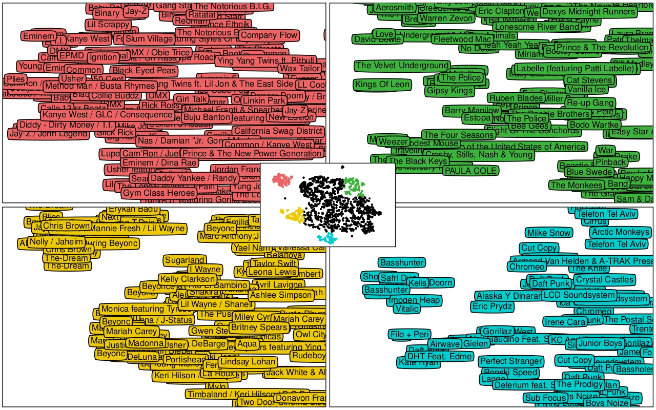
We visualized this in the paper by projecting the predictions of our model in the latent space down to two dimensions using the t-SNE algorithm. As you can see below on the resulting map, similar songs cluster together. Rap music can be found mostly in the top left corner, whereas electronic artists congregate at the bottom of the map.
t-SNE visualization of the latent space (middle). A few close-ups show artists whose songs are projected in specific areas. Taken from Deep content-based music recommendation, Aäron van den Oord, Sander Dieleman and Benjamin Schrauwen, NIPS 2013.
Scaling up
The deep neural network that we trained for the paper consisted of two convolutional layers and two fully connected layers. The input consisted of spectrograms of 3 second fragments of audio. To get a prediction for a longer clip, we just split it up into 3 second windows and averaged the predictions across these windows.
At Spotify, I have access to a larger dataset of songs, and a bunch of different latent factor representations obtained from various collaborative filtering models. They also got me a nice GPU to run my experiments on. This has allowed me to scale things up quite a bit. I am currently training convolutional neural networks (convnets) with 7 or 8 layers in total, using much larger intermediate representations and many more parameters.
Architecture
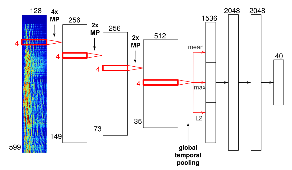
Below is an example of an architecture that I’ve tried out, which I will describe in more detail. It has four convolutional layers and three dense layers. As you will see, there are some important differences between convnets designed for audio signals and their more traditional counterparts used for computer vision tasks.
Warning: gory details ahead! Feel free to skip ahead to ‘Analysis’ if you don’t care about things like ReLUs, max-pooling and minibatch gradient descent.
One of the convolutional neural network architectures I've tried out for latent factor prediction. The time axis (which is convolved over) is vertical.
The input to the network consists of mel-spectrograms, with 599 frames and 128 frequency bins. A mel-spectrograms is a kind of time-frequency representation. It is obtained from an audio signal by computing the Fourier transforms of short, overlapping windows. Each of these Fourier transforms constitutes a frame. These successive frames are then concatenated into a matrix to form the spectrogram. Finally, the frequency axis is changed from a linear scale to a mel scale to reduce the dimensionality, and the magnitudes are scaled logarithmically.
The convolutional layers are displayed as red rectangles delineating the shape of the filters that slide across their inputs. They have rectified linear units (ReLUs, with activation function max(0, x)). Note that all these convolutions are one-dimensional; the convolution happens only in the time dimension, not in the frequency dimension. Although it is technically possible to convolve along both axes of the spectrogram, I am not currently doing this. It is important to realize that the two axes of a spectrogram have different meanings (time vs. frequency), which is not the case for images. As a result, it doesn’t really make sense to use square filters, which is what is typically done in convnets for image data.
Between the convolutional layers, there are max-pooling operations to downsample the intermediate representations in time, and to add some time invariance in the process. These are indicated with ‘MP’. As you can see I used a filter size of 4 frames in every convolutional layer, with max-pooling with a pool size of 4 between the first and second convolutional layers (mainly for performance reasons), and with a pool size of 2 between the other layers.
After the last convolutional layer, I added a global temporal pooling layer. This layer pools across the entire time axis, effectively computing statistics of the learned features across time. I included three different pooling functions: the mean, the maximum and the L2-norm.
I did this because the absolute location of features detected in the audio signal is not particularly relevant for the task at hand. This is not the case in image classification: in an image, it can be useful to know roughly where a particular feature was detected. For example, a feature detecting clouds would be more likely to activate for the top half of an image. If it activates in the bottom half, maybe it is actually detecting a sheep instead. For music recommendation, we are typically only interested in the overall presence or absence of certain features in the music, so it makes sense to perform pooling across time.
Another way to approach this problem would be to train the network on short audio fragments, and average the outputs across windows for longer fragments, as we did in the NIPS paper. However, incorporating the pooling into the model seems like a better idea, because it allows for this step to be taken into account during learning.
The globally pooled features are fed into a series of fully-connected layers with 2048 rectified linear units. In this network, I have two of them. The last layer of the network is the output layer, which predicts 40 latent factors obtained from the vector_exp algorithm, one of the various collaborative filtering algorithms that are used at Spotify.
Training
The network is trained to minimize the mean squared error (MSE) between the latent factor vectors from the collaborative filtering model and the predictions from audio. These vectors are first normalized so they have a unit norm. This is done to reduce the influence of song popularity (the norms of latent factor vectors tend to be correlated with song popularity for many collaborative filtering models). Dropout is used in the dense layers for regularization.
The dataset I am currently using consists of mel-spectrograms of 30 second excerpts extracted from the middle of the 1 million most popular tracks on Spotify. I am using about half of these for training (0.5M), about 5000 for online validation, and the remainder for testing. During training, the data is augmented by slightly cropping the spectrograms along the time axis with a random offset.
The network is implemented in Theano, and trained using minibatch gradient descent with Nesterov momentum on a NVIDIA GeForce GTX 780Ti GPU. Data loading and augmentation happens in a separate process, so while the GPU is training on a chunk of data, the next one can be loaded in parallel. About 750000 gradient updates are performed in total. I don’t remember exactly how long this particular architecture took to train, but all of the ones I’ve tried have taken between 18 and 36 hours.
Variations
As I mentioned before, this is just one example of an architecture that I’ve tried. Some other things I have tried / will try include:
Using maxout units instead of rectified linear units.
Using stochastic pooling instead of max-pooling.
Incorporating L2 normalization into the output layer of the network.
Data augmentation by stretching or compressing the spectrograms across time.
Concatenating multiple latent factor vectors obtained from different collaborative filtering models.
Here are some things that didn’t work quite as well as I’d hoped:
Adding ‘bypass’ connections from all convolutional layers to the fully connected part of the network, with global temporal pooling in between. The underlying assumption was that statistics about low-level features could also be useful for recommendation, but unfortunately this hampered learning too much.
Predicting the conditional variance of the factors as in mixture density networks, to get confidence estimates for the predictions and to identify songs for which latent factor prediction is difficult. Unfortunately this seemed to make training quite a lot harder, and the resulting confidence estimates did not behave as expected.
Analysis: what is it learning?
Now for the cool part: what are these networks learning? What do the features look like? The main reason I chose to tackle this problem with convnets, is because I believe that music recommendation from audio signals is a pretty complex problem bridging many levels of abstraction. My hope was that successive layers of the network would learn progressively more complex and invariant features, as they do for image classification problems.
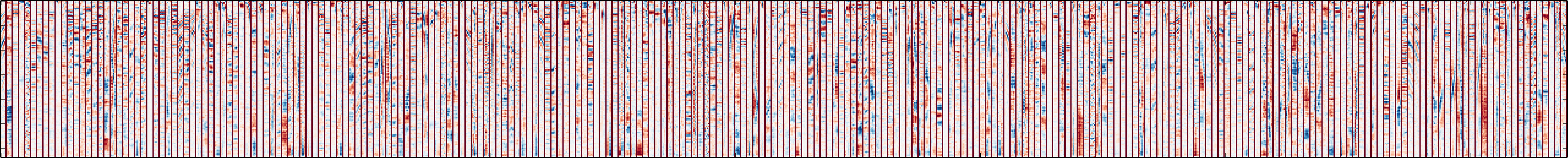
It looks like that’s exactly what is happening. First, let’s take a look at the first convolutional layer, which learns a set of filters that are applied directly to the input spectrograms. These filters are easy to visualize. They are shown in the image below. Click for a high resolution version (5584x562, ~600kB). Negative values are red, positive values are blue and white is zero. Note that each filter is only four frames wide. The individual filters are separated by dark red vertical lines.
Visualization of the filters learned in the first convolutional layer. The time axis is horizontal, the frequency axis is vertical (frequency increases from top to bottom). Click for a high resolution version (5584x562, ~600kB).
From this representation, we can see that a lot of the filters pick up harmonic content, which manifests itself as parallel red and blue bands at different frequencies. Sometimes, these bands are are slanted up or down, indicating the presence of rising and falling pitches. It turns out that these filters tend to detect human voices.
Playlists for low-level features: maximal activation
To get a better idea of what the filters learn, I made some playlists with songs from the test set that maximally activate them. Below are a few examples. There are 256 filters in the first layer of the network, which I numbered from 0 to 255. Note that this numbering is arbitrary, as they are unordered.
These four playlists were obtained by finding songs that maximally activate a given filter in the 30 seconds that were analyzed. I selected a few interesting looking filters from the first convolutional layer and computed the feature representations for each of these, and then searched for the maximal activations across the entire test set. Note that you should listen to the middle of the tracks to hear what the filters are picking up on, as this is the part of the audio signal that was analyzed.
All of the Spotify playlists below should have 10 tracks. Some of them may not be available in all countries due to licensing issues.
Filter 14: vibrato singing
Filter 242: ambience
Filter 250: vocal thirds
Filter 253: bass drums
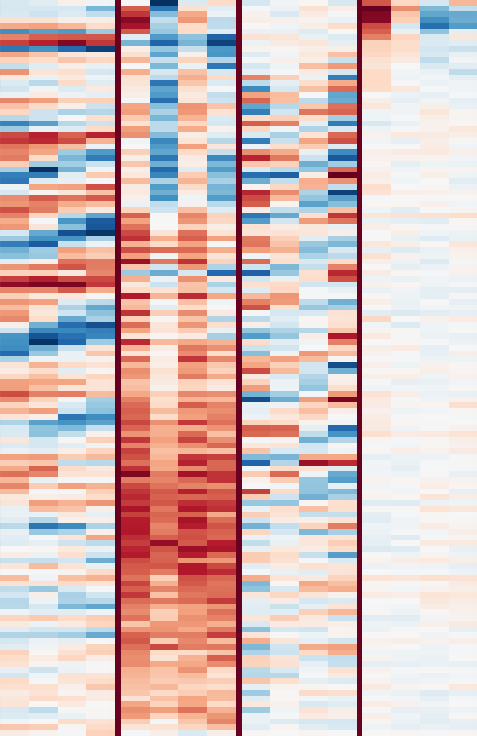
Closeup of filters 14, 242, 250 and 253. Click for a larger version.
Filter 14 seems to pick up vibrato singing.
Filter 242 picks up some kind of ringing ambience.
Filter 250 picks up vocal thirds, i.e. multiple singers singing the same thing, but the notes are a major third (4 semitones) apart.
Filter 253 picks up various types of bass drum sounds.
The genres of the tracks in these playlists are quite varied, which indicates that these features are picking up mainly low-level properties of the audio signals.
Playlists for low-level features: average activation
The next four playlists were obtained in a slightly different way: I computed the average activation of each feature across time for each track, and then found the maximum across those. This means that for these playlists, the filter in question is constantly active in the 30 seconds that were analyzed (i.e. it’s not just one ‘peak’). This is more useful for detecting harmonic patterns.
Filter 1: noise, distortion
Filter 2: pitch (A, Bb)
Filter 4: drones
Filter 28: chord (A, Am)
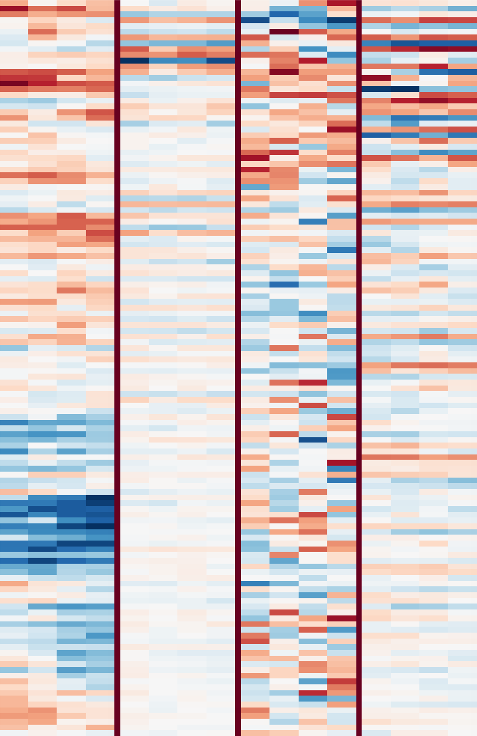
Closeup of filters 1, 2, 4 and 28. Click for a larger version.
Filter 1 picks up noise and (guitar) distortion.
Filter 2 seems to pick up a specific pitch: a low Bb. It also picks up A sometimes (a semitone below) because the frequency resolution of the mel-spectrograms is not high enough to distinguish them.
Filter 4 picks up various low-pitched drones.
Filter 28 picks up the A chord. It seems to pick up both the minor and major versions, so it might just be detecting the pitches A and E (the fifth).
I thought it was very interesting that the network is learning to detect specific pitches and chords. I had previously assumed that the exact pitches or chords occurring in a song would not really affect listener preference. I have two hypotheses for why this might be happening:
The network is just learning to detect harmonicity, by learning various filters for different kinds of harmonics. These are then pooled together at a higher level to detect harmonicity across different pitches.
The network is learning that some chords and chord progressions are more common than others in certain genres of music.
I have not tried to verify either of these, but it seems like the latter would be pretty challenging for the network to pick up on, so I think the former is more likely.
Playlists for high-level features
Each layer in the network takes the feature representation from the layer below, and extracts a set of higher-level features from it. At the topmost fully-connected layer of the network, just before the output layer, the learned filters turn out to be very selective for certain subgenres. For obvious reasons, it is non-trivial to visualize what these filters pick up on at the spectrogram level. Below are six playlists with songs from the test set that maximally activate some of these high-level filters.
Filter 3: christian rock
Filter 15: choirs / a cappella + smooth jazz
Filter 26: gospel
Filter 37: Chinese pop
Filter 49: chiptune, 8-bit
Filter 1024: deep house
It is clear that each of these filters is identifying specific genres. Interestingly some filters, like #15 for example, seem to be multimodal: they activate strongly for two or more styles of music, and those styles are often completely unrelated. Presumably the output of these filters is disambiguated when viewed in combination with the activations of all other filters.
Filter 37 is interesting because it almost seems like it is identifying the Chinese language. This is not entirely impossible, since the phoneme inventory of Chinese is quite distinct from other languages. A few other seemingly language-specific filters seem to be learned: there is one that detects rap music in Spanish, for example. Another possibility is that Chinese pop music has some other characteristic that sets it apart, and the model is picking up on that instead.
I spent some time analyzing the first 50 or so filters in detail. Some other filter descriptions I came up with are: lounge, reggae, darkwave, country, metalcore, salsa, Dutch and German carnival music, children’s songs, dance, vocal trance, punk, Turkish pop, and my favorite, ‘exclusively Armin van Buuren’. Apparently he has so many tracks that he gets his own filter.
The filters learned by Alex Krizhevsky’s ImageNet network have been reused for various other computer vision tasks with great success. Based on their diversity and invariance properties, it seems that these filters learned from audio signals may also be useful for other music information retrieval tasks besides predicting latent factors.
Similarity-based playlists
Predicted latent factor vectors can be used to find songs that sound similar. Below are a couple of playlists that were generated by predicting the factor vector for a given song, and then finding other songs in the test set whose predicted factor vectors are close to it in terms of cosine distance. As a result, the first track in the playlist is always the query track itself.
The Notorious B.I.G. - Juicy (hip hop)
Cloudkicker - He would be riding on the subway... (post-rock, post-metal)
Architects - Numbers Count For Nothing (metalcore, hardcore)
Neophyte - Army of Hardcore (hardcore techno, gabber)
Fleet Foxes - Sun It Rises (indie folk)
John Coltrane - My Favorite Things (jazz)
Most of the similar tracks are pretty decent recommendations for fans of the query tracks. Of course these lists are far from perfect, but considering that they were obtained based only on the audio signals, the results are pretty decent. One example where things go wrong is the list for ‘My Favorite Things’ by John Coltrane, which features a couple of strange outliers, most notably ‘Crawfish’ by Elvis Presley. This is probably because the part of the audio signal that was analyzed (8:40 to 9:10) contains a crazy sax solo. Analyzing the whole song might give better results.
What will this be used for?
Spotify already uses a bunch of different information sources and algorithms in their recommendation pipeline, so the most obvious application of my work is simply to include it as an extra signal. However, it could also be used to filter outliers from recommendations made by other algorithms. As I mentioned earlier, collaborative filtering algorithms will tend to include intro tracks, outro tracks, cover songs and remixes in their recommendations. These could be filtered out effectively using an audio-based approach.
One of my main goals with this work is to make it possible to recommend new and unpopular music. I hope that this will help lesser known and up and coming bands, and that it will level the playing field somewhat by enabling Spotify to recommend their music to the right audience. (Promoting up and coming bands also happens to be one of the main objectives of my non-profit website got-djent.com.)
Hopefully some of this will be ready for A/B testing soon, so we can find out if these audio-based recommendations actually make a difference in practice. This is something I’m very excited about, as it’s not something you can easily do in academia.
Future work
Another type of user feedback that Spotify collects are the thumbs up and thumbs down that users can give to tracks played on radio stations. This type of information is very useful to determine which tracks are similar. Unfortunately, it is also quite noisy. I am currently trying to use this data in a ‘learning to rank’ setting. I’ve also been experimenting with various distance metric learning schemes, such as DrLIM. If anything cool comes out of that I might write another post about it.
Conclusion
In this post I’ve given an overview of my work so far as a machine learning intern at Spotify. I’ve explained my approach to using convnets for audio-based music recommendation and I’ve tried to provide some insight into what the networks actually learn. For more details about the approach, please refer to the NIPS 2013 paper ‘Deep content-based music recommendation’ by Aäron van den Oord and myself.
If you are interested in deep learning, feature learning and its applications to music, have a look at my research page for an overview of some other work I have done in this domain. If you’re interested in Spotify’s approach to music recommendation, check out thesepresentations on Slideshare and Erik Bernhardsson’s blog.
Spotify is a really cool place to work at. They are very open about their methods (and they let me write this blog post), which is not something you come across often in industry. If you are interested in recommender systems, collaborative filtering and/or music information retrieval, and you’re looking for an internship or something more permanent, don’t hesitate to get in touch with them.
If you have any questions or feedback about this post, feel free to leave a comment!
The three papers I discussed in the first part of the talk are described here, download links to the PDFs are included. A detailed description of my solution for the Galaxy Challenge is available in an earlier post on this blog. The code for all 17 models included in the winning ensemble is available on GitHub.


