
Classifier-free diffusion guidance1 dramatically improves samples produced by conditional diffusion models at almost no cost. It is simple to implement and extremely effective. It is also an essential component of OpenAI’s DALL·E 22 and Google’s Imagen3, powering their spectacular image generation results. In this blog post, I share my perspective and try to give some intuition about how it works.
Diffusion guidance
Barely two years ago, they were a niche interest on the fringes of generative modelling research, but today, diffusion models are the go-to model class for image and audio generation. In my previous blog post, I discussed the link between diffusion models and autoencoders. If you are unfamiliar with diffusion models, I recommend reading at least the first section of that post for context, before reading the rest of this one.
Diffusion models are generative models, which means they model a high-dimensional data distribution \(p(x)\). Rather than trying to approximate \(p(x)\) directly (which is what likelihood-based models do), they try to predict the so-called score function, \(\nabla_x \log p(x)\).
To sample from a diffusion model, an input is initialised to random noise, and is then iteratively denoised by taking steps in the direction of the score function (i.e. the direction in which the log-likelihood increases fastest), with some additional noise mixed in to avoid getting stuck in modes of the distribution. This is called Stochastic Gradient Langevin Dynamics (SGLD). This is a bit of a caricature of what people actually use in practice nowadays, but it’s not too far off the truth.
In conditional diffusion models, we have an additional input \(y\) (for example, a class label or a text sequence) and we try to model the conditional distribution \(p(x \mid y)\) instead. In practice, this means learning to predict the conditional score function \(\nabla_x \log p(x \mid y)\).
One neat aspect of the score function is that it is invariant to normalisation of the distribution: if we only know the distribution \(p(x)\) up to a constant, i.e. we have \(p(x) = \frac{\tilde{p}(x)}{Z}\) and we only know \(\tilde{p}(x)\), then we can still compute the score function:
\[\nabla_x \log \tilde{p}(x) = \nabla_x \log \left( p(x) \cdot Z \right) = \nabla_x \left( \log p(x) + \log Z \right) = \nabla_x \log p(x),\]where we have made use of the linearity of the gradient operator, and the fact that the normalisation constant \(Z = \int \tilde{p}(x) \mathrm{d} x\) does not depend on \(x\) (so its derivative w.r.t. \(x\) is zero).
Unnormalised probability distributions come up all the time, so this is a useful property. For conditional models, it enables us to apply Bayes’ rule to decompose the score function into an unconditional component, and a component that “mixes in” the conditioning information:
\[p(x \mid y) = \frac{p(y \mid x) \cdot p(x)}{p(y)}\] \[\implies \log p(x \mid y) = \log p(y \mid x) + \log p(x) - \log p(y)\] \[\implies \nabla_x \log p(x \mid y) = \nabla_x \log p(y \mid x) + \nabla_x \log p(x) ,\]where we have used that \(\nabla_x \log p(y) = 0\). In other words, we can obtain the conditional score function as simply the sum of the unconditional score function and a conditioning term. (Note that the conditioning term \(\nabla_x \log p(y \mid x)\) is not itself a score function, because the gradient is w.r.t. \(x\), not \(y\).)
Throughout this blog post, I have mostly ignored the time dependency of the distributions estimated by diffusion models. This saves me having to add extra conditioning variables and subscripts everywhere. In practice, diffusion models perform iterative denoising, and are therefore usually conditioned on the level of input noise at each step.
Classifier guidance
The first thing to notice is that \(p(y \mid x)\) is exactly what classifiers and other discriminative models try to fit: \(x\) is some high-dimensional input, and \(y\) is a target label. If we have a differentiable discriminative model that estimates \(p(y \mid x)\), then we can also easily obtain \(\nabla_x \log p(y \mid x)\). All we need to turn an unconditional diffusion model into a conditional one, is a classifier!
The observation that diffusion models can be conditioned post-hoc in this way was mentioned by Sohl-Dickstein et al.4 and Song et al.5, but Dhariwal and Nichol6 really drove this point home, and showed how classifier guidance can dramatically improve sample quality by enhancing the conditioning signal, even when used in combination with traditional conditional modelling. To achieve this, they scale the conditioning term by a factor:
\[\nabla_x \log p_\gamma(x \mid y) = \nabla_x \log p(x) + \gamma \nabla_x \log p(y \mid x) .\]\(\gamma\) is called the guidance scale, and cranking it up beyond 1 has the effect of amplifying the influence of the conditioning signal. It is extremely effective, especially compared to e.g. the truncation trick for GANs7, which serves a similar purpose.

If we revert the gradient and the logarithm operations that we used to go from Bayes’ rule to classifier guidance, it’s easier to see what’s going on:
\[p_\gamma(x \mid y) \propto p(x) \cdot p(y \mid x)^\gamma .\]We are raising the conditional part of the distribution to a power, which corresponds to tuning the temperature of that distribution: \(\gamma\) is an inverse temperature parameter. If \(\gamma > 1\), this sharpens the distribution and focuses it onto its modes, by shifting probability mass from the least likely to the most likely values (i.e. the temperature is lowered). Classifier guidance allows us to apply this temperature tuning only to the part of the distribution that captures the influence of the conditioning signal.
In language modelling, it is now commonplace to train a powerful unconditional language model once, and then adapt it to downstream tasks as needed (via few-shot learning or finetuning). Superficially, it would seem that classifier guidance enables the same thing for image generation: one could train a powerful unconditional model, then condition it as needed at test time using a separate classifier.
Unfortunately there are a few snags that make this impractical. Most importantly, because diffusion models operate by gradually denoising inputs, any classifier used for guidance also needs to be able to cope with high noise levels, so that it can provide a useful signal all the way through the sampling process. This usually requires training a bespoke classifier specifically for the purpose of guidance, and at that point, it might be easier to train a traditional conditional generative model end-to-end (or at least finetune an unconditional model to incorporate the conditioning signal).
But even if we have a noise-robust classifier on hand, classifier guidance is inherently limited in its effectiveness: most of the information in the input \(x\) is not relevant to predicting \(y\), and as a result, taking the gradient of the classifier w.r.t. its input can yield arbitrary (and even adversarial) directions in input space.
Classifier-free guidance
This is where classifier-free guidance1 comes in. As the name implies, it does not require training a separate classifier. Instead, one trains a conditional diffusion model \(p(x \mid y)\), with conditioning dropout: some percentage of the time, the conditioning information \(y\) is removed (10-20% tends to work well). In practice, it is often replaced with a special input value representing the absence of conditioning information. The resulting model is now able to function both as a conditional model \(p(x \mid y)\), and as an unconditional model \(p(x)\), depending on whether the conditioning signal is provided. One might think that this comes at a cost to conditional modelling performance, but the effect seems to be negligible in practice.
What does this buy us? Recall Bayes’ rule from before, but let’s apply it in the other direction:
\[p(y \mid x) = \frac{p(x \mid y) \cdot p(y)}{p(x)}\] \[\implies \log p(y \mid x) = \log p(x \mid y) + \log p(y) - \log p(x)\] \[\implies \nabla_x \log p(y \mid x) = \nabla_x \log p(x \mid y) - \nabla_x \log p(x) .\]We have expressed the conditioning term as a function of the conditional and unconditional score functions, both of which our diffusion model provides. We can now substitute this into the formula for classifier guidance:
\[\nabla_x \log p_\gamma(x \mid y) = \nabla_x \log p(x) + \gamma \left( \nabla_x \log p(x \mid y) - \nabla_x \log p(x) \right),\]or equivalently:
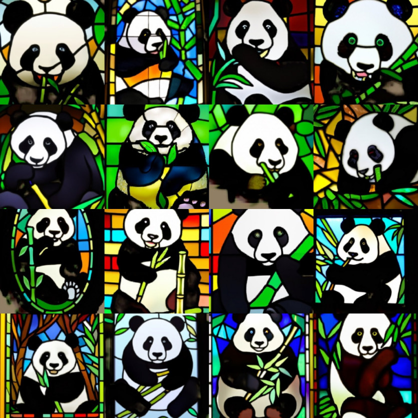
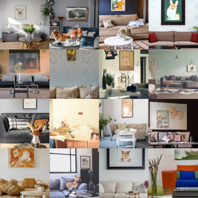
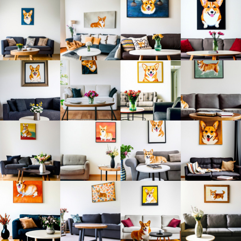
\[\nabla_x \log p_\gamma(x \mid y) = (1 - \gamma) \nabla_x \log p(x) + \gamma \nabla_x \log p(x \mid y) .\]This is a barycentric combination of the conditional and the unconditional score function. For \(\gamma = 0\), we recover the unconditional model, and for \(\gamma = 1\) we get the standard conditional model. But \(\gamma > 1\) is where the magic happens. Below are some examples from OpenAI’s GLIDE model8, obtained using classifier-free guidance.
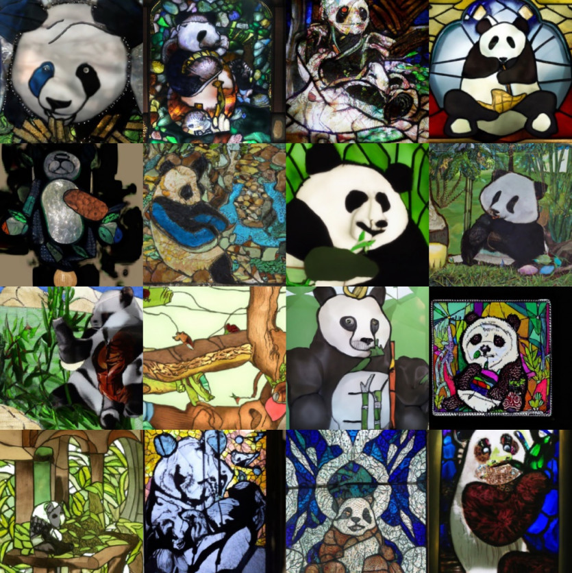
Why does this work so much better than classifier guidance? The main reason is that we’ve constructed the “classifier” from a generative model. Whereas standard classifiers can take shortcuts and ignore most of the input \(x\) while still obtaining competitive classification results, generative models are afforded no such luxury. This makes the resulting gradient much more robust. As a bonus, we only have to train a single (generative) model, and conditioning dropout is trivial to implement.
It is worth noting that there was only a very brief window of time between the publication of the classifier-free guidance idea, and OpenAI’s GLIDE model, which used it to great effect – so much so that the idea has sometimes been attributed to the latter! Simple yet powerful ideas tend to see rapid adoption. In terms of power-to-simplicity ratio, classifier-free guidance is up there with dropout9, in my opinion: a real game changer!
(In fact, the GLIDE paper says that they originally trained a text-conditional model, and applied conditioning dropout only in a finetuning phase. Perhaps there is a good reason to do it this way, but I rather suspect that this is simply because they decided to apply the idea to a model they had already trained before!)
Clearly, guidance represents a trade-off: it dramatically improves adherence to the conditioning signal, as well as overall sample quality, but at great cost to diversity. In conditional generative modelling, this is usually an acceptable trade-off, however: the conditioning signal often already captures most of the variability that we actually care about, and if we desire diversity, we can also simply modify the conditioning signal we provide.
Guidance for autoregressive models
Is guidance unique to diffusion models? On the face of it, not really. People have pointed out that you can do similar things with other model classes:
You can apply a similar trick to classifier-free guidance to autoregressive transformers to sample from a synthetic "super-conditioned" distribution. I trained a CIFAR-10 class-conditional ImageGPT to try this, and I got the following grids with cond_scale 1 (default) and then 3: pic.twitter.com/gWL5sOqXck
— Rivers Have Wings (@RiversHaveWings) January 3, 2022
You can train autoregressive models with conditioning dropout just as easily, and then use two sets of logits produced with and without conditioning to construct classifier-free guided logits, just as we did before with score functions. Whether we apply this operation to log-probabilities or gradients of log-probabilities doesn’t really make a difference, because the gradient operator is linear.
There is an important difference however: whereas the score function in a diffusion model represents the joint distribution across all components of \(x\), \(p(x \mid y)\), the logits produced by autoregressive models represent \(p(x_t \mid x_{<t}, y)\), the sequential conditional distributions. You can obtain a joint distribution \(p(x \mid y)\) from this by multiplying all the conditionals together:
\[p(x \mid y) = \prod_{t=1}^T p(x_t \mid x_{<t}, y),\]but guidance on each of the factors of this product is not equivalent to applying it to the joint distribution, as one does in diffusion models:
\[p_\gamma(x \mid y) \neq \prod_{t=1}^T p_\gamma(x_t \mid x_{<t}, y).\]To see this, let’s first expand the left hand side:
\[p_\gamma(x \mid y) = \frac{p(x) \cdot p(y \mid x)^\gamma}{\int p(x) \cdot p(y \mid x)^\gamma \mathrm{d} x},\]from which we can divide out the unconditional distribution \(p(x)\) to obtain an input-dependent scale factor that adapts the probabilities based on the conditioning signal \(y\):
\[s_\gamma(x, y) := \frac{p(y \mid x)^\gamma}{\mathbb{E}_{p(x)}\left[ p(y \mid x)^\gamma \right]} .\]Now we can do the same thing with the right hand side:
\[\prod_{t=1}^T p_\gamma(x_t \mid x_{<t}, y) = \prod_{t=1}^T \frac{p(x_t \mid x_{<t}) \cdot p(y \mid x_{\le t})^\gamma}{\int p(x_t \mid x_{<t}) \cdot p(y \mid x_{\le t})^\gamma \mathrm{d} x_t}\]We can again factor out \(p(x)\) here:
\[\prod_{t=1}^T p_\gamma(x_t \mid x_{<t}, y) = p(x) \cdot \prod_{t=1}^T \frac{p(y \mid x_{\le t})^\gamma}{\int p(x_t \mid x_{<t}) \cdot p(y \mid x_{\le t})^\gamma \mathrm{d} x_t}.\]The input-dependent scale factor is now:
\[s_\gamma'(x, y) := \prod_{t=1}^T \frac{p(y \mid x_{\le t})^\gamma}{ \mathbb{E}_{p(x_t \mid x_{<t})} \left[ p(y \mid x_{\le t})^\gamma \right] },\]which is clearly not equivalent to \(s_\gamma(x, y)\). In other words, guidance on the sequential conditionals redistributes the probability mass in a different way than guidance on the joint distribution does.
I don’t think this has been extensively tested at this point, but my hunch is that diffusion guidance works so well precisely because we are able to apply it to the joint distribution, rather than to individual sequential conditional distributions. As of today, diffusion models are the only model class for which this approach is tractable (if there are others, I’d be very curious to learn about them, so please share in the comments!).
As an aside: if you have an autoregressive model where the underlying data can be treated as continuous (e.g. an autoregressive model of images like PixelCNN10 or an Image Transformer11), you can actually get gradients w.r.t. the input. This means you can get an efficient estimate of the score function \(\nabla_x \log p(x|y)\) and sample from the model using Langevin dynamics, so you could in theory apply classifier or classifier-free guidance to the joint distribution, in a way that’s equivalent to diffusion guidance!
Update / correction (May 29th)
@RiversHaveWings on Twitter pointed out that the distributions which we modify to apply guidance are \(p_t(x \mid y)\) (where \(t\) is the current timestep in the diffusion process), not \(p(x \mid y)\) (which is equivalent to \(p_0(x \mid y)\)). This is clearly a shortcoming of the notational shortcut I took throughout this blog post (i.e. making the time dependency implicit).
This calls into question my claim above that diffusion model guidance operates on the true joint distribution of the data – though it doesn’t change the fact that guidance does a different thing for autoregressive models and for diffusion models. As ever in deep learning, whether the difference is meaningful in practice will probably have to be established empirically, so it will be interesting to see if classifier-free guidance catches on for other model classes as well!
Temperature tuning for diffusion models
One thing people often do with autoregressive models is tune the temperature of the sequential conditional distributions. More intricate procedures to “shape” these distributions are also popular: top-k sampling, nucleus sampling12 and typical sampling13 are the main contenders. They are harder to generalise to high-dimensional distributions, so I won’t consider them here.
Can we tune the temperature of a diffusion model? Sure: instead of factorising \(p(x \mid y)\) and only modifying the conditional component, we can just raise the whole thing to the \(\gamma\)‘th power simply by multiplying the score function with \(\gamma\). Unfortunately, this invariably yields terrible results. While tuning temperatures of the sequential conditionals in autoregressive models works quite well, and often yields better results, tuning the temperature of the joint distribution seems to be pretty much useless (let me know in the comments if your experience differs!).
Just as with guidance, this is because changing the temperature of the sequential conditionals is not the same as changing the temperature of the joint distribution. Working this out is left as an excerise to the reader :)
Note that they do become equivalent when all \(x_t\) are independent (i.e. \(p(x_t \mid x_{<t}) = p(x_t)\)), but if that is the case, using an autoregressive model kind of defeats the point!
Closing thoughts

Guidance is far from the only reason why diffusion models work so well for images: the standard loss function for diffusion de-emphasises low noise levels, relative to the likelihood loss14. As I mentioned in my previous blog post, noise levels and image feature scales are closely tied together, and the result is that diffusion models pay less attention to high-frequency content that isn’t visually salient to humans anyway, enabling them to use their capacity more efficiently.
That said, I think guidance is probably the main driver behind the spectacular results we’ve seen over the course of the past six months. I believe guidance constitutes a real step change in our ability to generate perceptual signals, going far beyond the steady progress of the last few years that this domain has seen. It is striking that the state-of-the-art models in this domain are able to do what they do, while still being one to two orders of magnitude smaller than state-of-the-art language models in terms of parameter count.
I also believe we’ve only scratched the surface of what’s possible with diffusion models’ steerable sampling process. Dynamic thresholding, introduced this week in the Imagen paper3, is another simple guidance-enhancing trick to add to our arsenal, and I think there are many more such tricks to be discovered (as well as more elaborate schemes). Guidance seems like it might also enable a kind of “arithmetic” in the image domain like we’ve seen with word embeddings.
If you would like to cite this post in an academic context, you can use this BibTeX snippet:
@misc{dieleman2022guidance,
  author = {Dieleman, Sander},
  title = {Guidance: a cheat code for diffusion models},
  url = {https://benanne.github.io/2022/05/26/guidance.html},
  year = {2022}
}
Acknowledgements
Thanks to my colleagues at DeepMind for various discussions, which continue to shape my thoughts on this topic!
References
-
Ho, Salimans, “Classifier-Free Diffusion Guidance”, NeurIPS workshop on DGMs and Applications”, 2021. ↩ ↩2
-
Ramesh, Dhariwal, Nichol, Chu, Chen, “Hierarchical Text-Conditional Image Generation with CLIP Latents”, arXiv, 2022. ↩
-
Saharia, Chan, Saxena, Li, Whang, Ho, Fleet, Norouzi et al., “Photorealistic Text-to-Image Diffusion Models with Deep Language Understanding”, arXiv, 2022. ↩ ↩2
-
Sohl-Dickstein, Weiss, Maheswaranathan and Ganguli, “Deep Unsupervised Learning using Nonequilibrium Thermodynamics”, International Conference on Machine Learning, 2015. ↩
-
Song, Sohl-Dickstein, Kingma, Kumar, Ermon and Poole, “Score-Based Generative Modeling through Stochastic Differential Equations”, International Conference on Learning Representations, 2021. ↩
-
Dhariwal, Nichol, “Diffusion Models Beat GANs on Image Synthesis”, Neural Information Processing Systems, 2021. ↩
-
Brock, Donahue, Simonyan, “Large Scale GAN Training for High Fidelity Natural Image Synthesis”, International Conference on Learning Representations, 2019. ↩
-
Nichol, Dhariwal, Ramesh, Shyam, Mishkin, McGrew, Sutskever, Chen, “GLIDE: Towards Photorealistic Image Generation and Editing with Text-Guided Diffusion Models”, arXiv, 2021. ↩
-
Srivastava, Hinton, Krizhevsky, Sutskever, Salakhutdinov, “Dropout: A Simple Way to Prevent Neural Networks from Overfitting”, Journal of Machine Learning Research, 2014. ↩
-
Van den Oord, Kalchbrenner, Kavukcuoglu, “Pixel Recurrent Neural Networks”, International Conference on Machine Learning, 2016. ↩
-
Parmar, Vaswani, Uszkoreit, Kaiser, Shazeer, Ku, Tran, “Image Transformer”, International Conference on Machine Learning, 2018. ↩
-
Holtzman, Buys, Du, Forbes, Choi, “The Curious Case of Neural Text Degeneration”, International Conference on Learning Representations, 2020. ↩
-
Meister, Pimentel, Wiher, Cotterell, “Typical Decoding for Natural Language Generation”, arXiv, 2022. ↩
-
Song, Durkan, Murray, Ermon, “Maximum Likelihood Training of Score-Based Diffusion Models”, Neural Information Processing Systems, 2021 ↩