The paradox of diffusion distillation

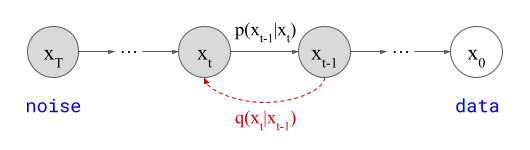
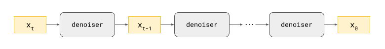
Diffusion models split up the difficult task of generating data from a high-dimensional distribution into many denoising tasks, each of which is much easier. We train them to solve just one of these tasks at a time. To sample, we make many predictions in sequence. This iterative refinement is where their power comes from.
…or is it? A lot of recent papers about diffusion models focus on reducing the number of sampling steps required; some works even aim to enable single-step sampling. That seems counterintuitive, when splitting things up into many easier steps is supposedly why these models work so well in the first place!

In this blog post, let’s take a closer look at the various ways in which the number of sampling steps required to get good results from diffusion models can be reduced. We will focus on various forms of distillation in particular: this is the practice of training a new model (the student) by supervising it with the predictions of another model (the teacher). Various distillation methods for diffusion models have produced extremely compelling results.

I intended this to be relatively high-level when I started writing, but since distillation of diffusion models is a bit of a niche subject, I could not avoid explaining certain things in detail, so it turned into a deep dive. Below is a table of contents. Click to jump directly to a particular section of this post.

  1. Diffusion sampling: tread carefully!
  2. Moving through input space with purpose
  3. Diffusion distillation
  4. But what about “no free lunch”?
  5. Do we really need a teacher?
  6. Charting the maze between data and noise
  7. Closing thoughts
  8. Acknowledgements
  9. References

Diffusion sampling: tread carefully!

First of all, why does it take many steps to get good results from a diffusion model? It’s worth developing a deeper understanding of this, in order to appreciate how various methods are able to cut down on this without compromising the quality of the output – or at least, not too much.

A sampling step in a diffusion model consists of:

  • predicting the direction in input space in which we should move to remove noise, or equivalently, to make the input more likely under the data distribution;
  • taking a small step in that direction.

Depending on the sampling algorithm, you might add a bit of noise, or use a more advanced mechanism to compute the update direction.

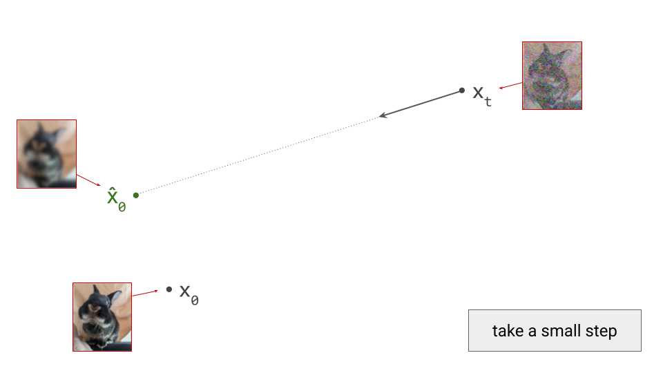
We only take a small step, because this predicted direction is only meaningful locally: it points towards a region of input space where the likelihood under the data distribution is high – not to any specific data point in particular. So if we were to take a big step, we would end up in the centroid of that high-likelihood region, which isn’t necessarily a representative sample of the data distribution. Think of it as a rough estimate. If you find this unintuitive, you are not alone! Probability distributions in high-dimensional spaces often behave unintuitively, something I’ve written an an in-depth blog post about in the past.

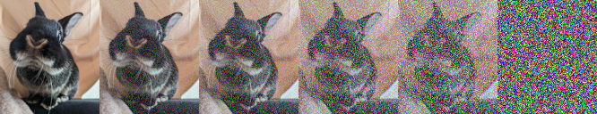
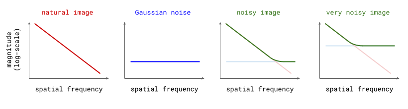
Concretely, in the image domain, taking a big step in the predicted direction tends to yield a blurry image, if there is a lot of noise in the input. This is because it basically corresponds to the average of many plausible images. (For the sake of argument, I am intentionally ignoring any noise that might be added back in as part of the sampling algorithm.)

Another way of looking at it is that the noise obscures high-frequency information, which corresponds to sharp features and fine-grained details (something I’ve also written about before). The uncertainty about this high-frequency information yields a prediction where all the possibilities are blended together, which results in a lack of high-frequency information altogether.

The local validity of the predicted direction implies we should only be taking infinitesimal steps, and then reevaluating the model to determine a new direction. Of course, this is not practical, so we take finite but small steps instead. This is very similar to the way gradient-based optimisation of machine learning models works in parameter space, but here we are operating in the input space instead. Just as in model training, if the steps we take are too large, the quality of the end result will suffer.

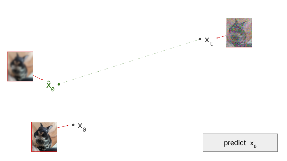
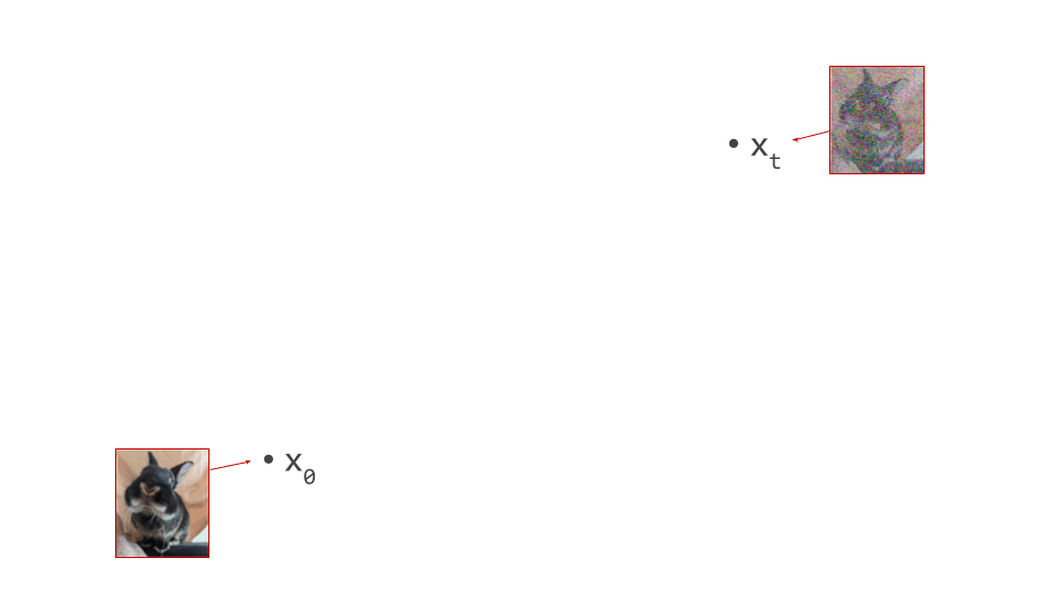
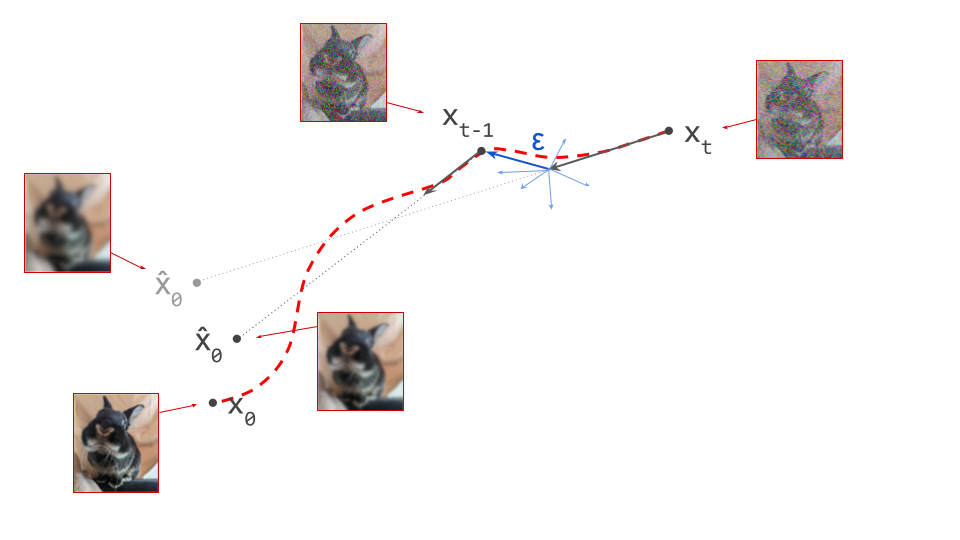
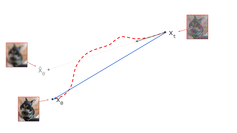
Below is a diagram that represents the input space in two dimensions. \(\mathbf{x}_t\) represents the noisy input at time step \(t\), which we constructed here by adding noise to a clean image \(\mathbf{x}_0\) drawn from the data distribution. Also shown is the direction (predicted by a diffusion model) in which we should move to make the input more likely. This points to \(\hat{\mathbf{x}}_0\), the centroid of a region of high likelihood, which is shaded in pink.

Diagram showing a region of high likelihood in input space, as well as the direction predicted by a diffusion model, which points to the centroid of this region.

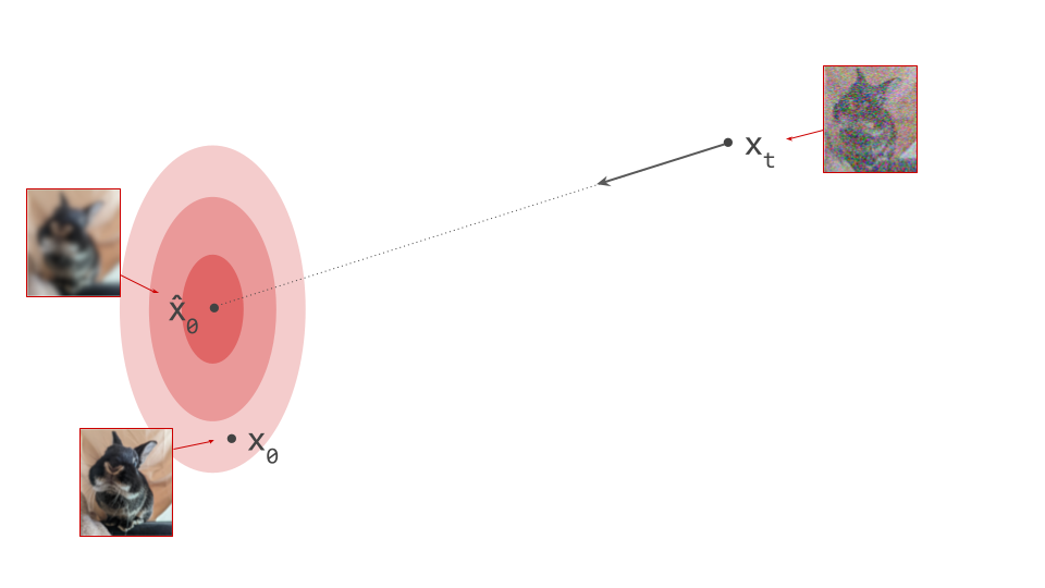
(Please see the first section of my previous blog post on the geometry of diffusion guidance for some words of caution about representing very high-dimensional spaces in 2D!)

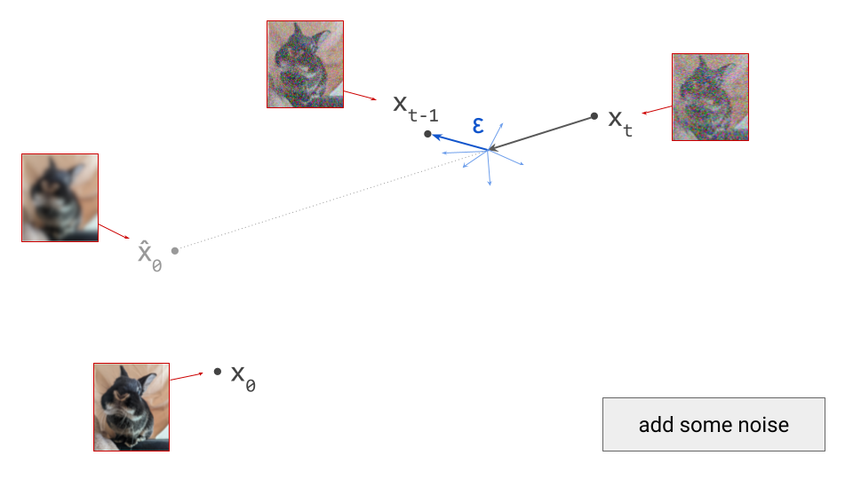
If we proceed to take a step in this direction and add some noise (as we do in the DDPM1 sampling algorithm, for example), we end up with \(\mathbf{x}_{t-1}\), which corresponds to a slightly less noisy input image. The predicted direction now points to a smaller, “more specific” region of high likelihood, because some uncertainty was resolved by the previous sampling step. This is shown in the diagram below.

Diagram showing the updated direction predicted by a diffusion model after a single sampling step, as well as the corresponding region of high likelihood which it points to.

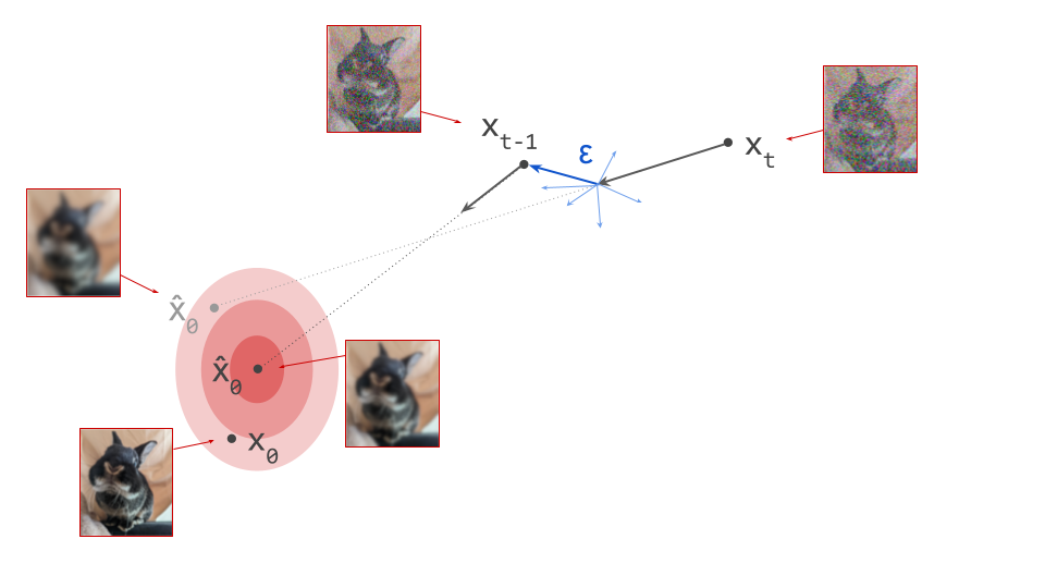
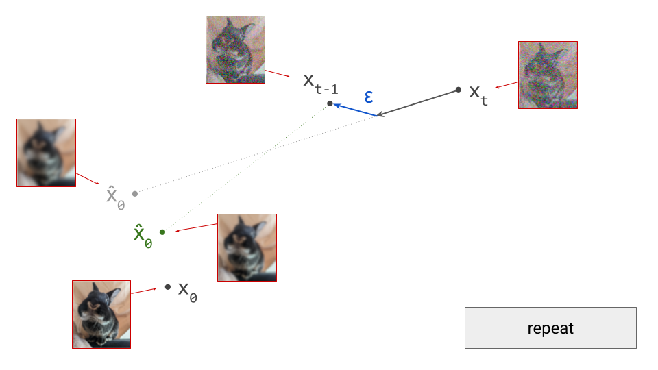
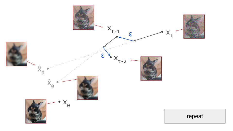
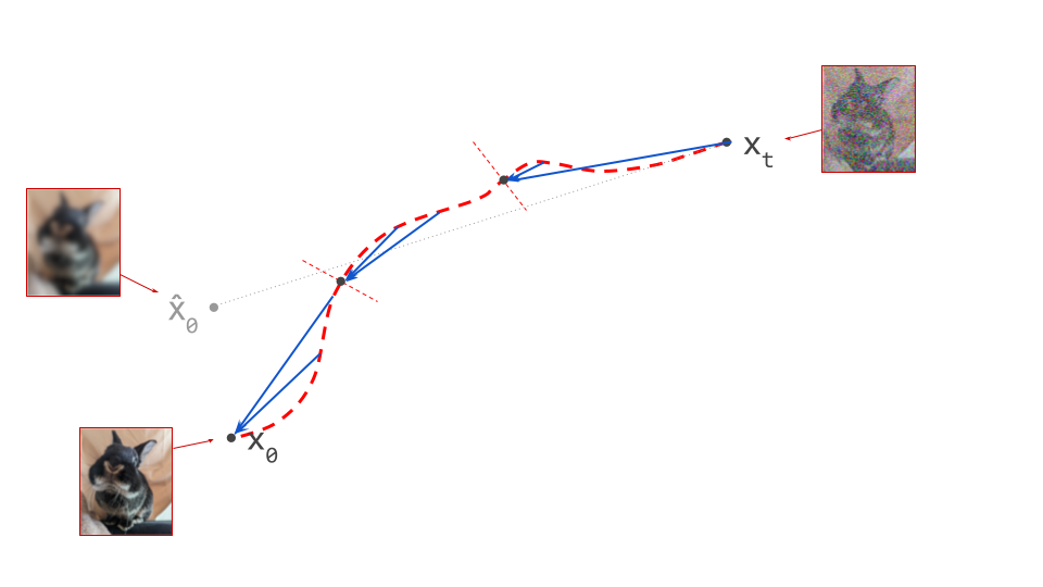
The change in direction at every step means that the path we trace out through input space during sampling is curved. Actually, because we are making a finite approximation, that’s not entirely accurate: it is actually a piecewise linear path. But if we let the number of steps go to infinity, we would end up with a curve. The predicted direction at each point on this curve corresponds to the tangent direction. A stylised version of what this curve might look like is shown in the diagram below.

Diagram showing a stylised version of the curve we might trace through input space with an infinite number of sampling steps (dashed red curve).

Moving through input space with purpose

A plethora of diffusion sampling algorithms have been developed to move through input space more swiftly and reduce the number of sampling steps required to achieve a certain level of output quality. Trying to list all of them here would be a hopeless endeavour, but I want to highlight a few of these algorithms to demonstrate that a lot of the ideas behind them mimic techniques used in gradient-based optimisation.

A very common question about diffusion sampling is whether we should be injecting noise at each step, as in DDPM1, and sampling algorithms based on stochastic differential equation (SDE) solvers2. Karras et al.3 study this question extensively (see sections 3 & 4 in their “instant classic” paper) and find that the main effect of introducing stochasticity is error correction: diffusion model predictions are approximate, and noise helps to prevent these approximation errors from accumulating across many sampling steps. In the context of optimisation, the regularising effect of noise in stochastic gradient descent (SGD) is well-studied, so perhaps this is unsurprising.

However, for some applications, injecting randomness at each sampling step is not acceptable, because a deterministic mapping between samples from the noise distribution and samples from the data distribution is necessary. Sampling algorithms such as DDIM4 and ODE-based approaches2 make this possible (I’ve previously written about this feat of magic, as well as how this links together diffusion models and flow-based models). An example of where this comes in handy is for teacher models in the context of distillation (see next section). In that case, other techniques can be used to reduce approximation error while avoiding an increase in the number of sampling steps.

One such technique is the use of higher order methods. Heun’s 2nd order method for solving differential equations results in an ODE-based sampler that requires two model evaluations per step, which it uses to obtain improved estimates of update directions5. While this makes each sampling step approximately twice as expensive, the trade-off can still be favourable in terms of the total number of function evaluations3.

Another variant of this idea involves making the model predict higher-order score functions – think of this as the model estimating both the direction and the curvature, for example. These estimates can then be used to move faster in regions of low curvature, and slow down appropriately elsewhere. GENIE6 is one such method, which involves distilling the expensive second order gradient calculation into a small neural network to reduce the additional cost to a practical level.

Finally, we can emulate the effect of higher-order information by aggregating information across sampling steps. This is very similar to the use of momentum in gradient-based optimisation, which also enables acceleration and deceleration depending on curvature, but without having to explicitly estimate second order quantities. In the context of differential equation solving, this approach is usually termed a multistep method, and this idea has inspired many diffusion sampling algorithms7 8 9 10.

In addition to the choice of sampling algorithm, we can also choose how to space the time steps at which we compute updates. These are spaced uniformly across the entire range by default (think np.linspace), but because noise schedules are often nonlinear (i.e. \(\sigma_t\) is a nonlinear function of \(t\)), the corresponding noise levels are spaced in a nonlinear fashion as a result. However, it can pay off to treat sampling step spacing as a hyperparameter to tune separately from the choice of noise schedule (or, equivalently, to change the noise schedule at sampling time). Judiciously spacing out the time steps can improve the quality of the result at a given step budget3.

Diffusion distillation

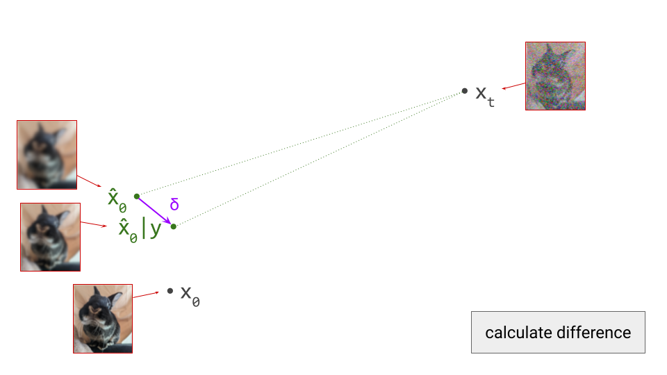
Broadly speaking, in the context of neural networks, distillation refers to training a neural network to mimic the outputs of another neural network11. The former is referred to as the student, while the latter is the teacher. Usually, the teacher has been trained previously, and its weights are frozen. When applied to diffusion models, something interesting happens: even if the student and teacher networks are identical in terms of architecture, the student will converge significantly faster than the teacher did when it was trained.

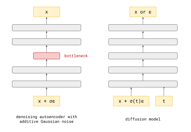
To understand why this happens, consider that diffusion model training involves supervising the network with examples \(\mathbf{x}_0\) from the dataset, to which we have added varying amounts of noise to create the network input \(\mathbf{x}_t\). But rather than expecting the network to be able to predict \(\mathbf{x}_0\) exactly, what we actually want is for it to predict \(\mathbb{E}\left[\mathbf{x}_0 \mid \mathbf{x}_t \right]\), that is, a conditional expectation over the data distribution. It’s worth revisiting the first diagram in section 1 of this post to grasp this: we supervise the model with \(\mathbf{x}_0\), but this is not what we want the model to predict – what we actually want is for it to predict a direction pointing to the centroid of a region of high likelihood, which \(\mathbf{x}_0\) is merely a representative sample of. I’ve previously mentioned this when discussing various perspectives on diffusion. This means that weight updates are constantly pulling the model weights in different directions as training progresses, slowing down convergence.

When we distill a diffusion model, rather than training it from scratch, the teacher provides an approximation of \(\mathbb{E}\left[\mathbf{x}_0 \mid \mathbf{x}_t \right]\), which the student learns to mimic. Unlike before, the target used to supervise the model is now already an (approximate) expectation, rather than a single representative sample. As a result, the variance of the distillation loss is significantly reduced compared to that of the standard diffusion training loss. Whereas the latter tends to produce training curves that are jumping all over the place, distillation provides a much smoother ride. This is especially obvious when you plot both training curves side by side. Note that this variance reduction does come at a cost: since the teacher is itself an imperfect model, we’re actually trading variance for bias.

Variance reduction alone does not explain why distillation of diffusion models is so popular, however. Distillation is also a very effective way to reduce the number of sampling steps required. It seems to be a lot more effective in this regard than simply changing up the sampling algorithm, but of course there is also a higher upfront cost, because it requires additional model training.

There are many variants of diffusion distillation, a few of which I will try to compactly summarise below. It goes without saying that this is not an exhaustive review of the literature. A relatively recent survey paper is Weijian Luo’s (from April 2023)12, though a lot of work has appeared in this space since then, so I will try to cover some newer things as well. If you feel there is a particular method that’s worth mentioning but that I didn’t cover, let me know in the comments.

Distilling diffusion sampling into a single forward pass

A typical diffusion sampling procedure involves repeatedly applying a neural network on a canvas, and using the prediction to update that canvas. When we unroll the computational graph of this network, this can be reinterpreted as a much deeper neural network in its own right, where many layers share weights. I’ve previously discussed this perspective on diffusion in more detail.

Distillation is often used to compress larger networks into smaller ones, so Luhman & Luhman13 set out to train a much smaller student network to reproduce the outputs of this much deeper teacher network corresponding to an unrolled sampling procedure. In fact, what they propose is to distill the entire sampling procedure into a network with the same architecture used for a single diffusion prediction step, by matching outputs in the least-squares sense (MSE loss). Depending on how many steps the sampling procedure has, this may correspond to quite an extreme form of model compression (in the sense of compute, that is – the number of parameters stays the same, of course).

This approach requires a deterministic sampling procedure, so they use DDIM4 – a choice which many distillation methods that were developed later also follow. The result of their approach is a compact student network which transforms samples from the noise distribution into samples from the data distribution in a single forward pass.

Diagram showing distillation of the diffusion sampling procedure into a single forward pass.

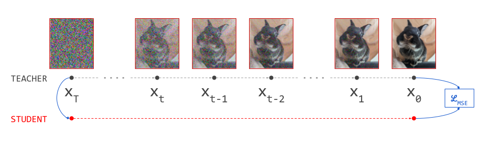
Putting this into practice, one encounters a significant hurdle, though: to obtain a single training example for the student, we have to run the full diffusion sampling procedure using the teacher, which is usually too expensive to do on-the-fly during training. Therefore the dataset for the student has to be pre-generated offline. This is still expensive, but at least it only has to be done once, and the resulting training examples can be reused for multiple epochs.

To speed up the learning process, it also helps to initialise the student with the weights of the teacher (which we can do because their architectures are identical). This is a trick that most diffusion distillation methods make use of.

This work served as a compelling proof-of-concept for diffusion distillation, but aside from the computational cost, the accumulation of errors in the deterministic sampling procedure, combined with the approximate nature of the student predictions, imposed significant limits on the achievable output quality.

Progressive distillation

Progressive distillation14 is an iterative approach that halves the number of required sampling steps. This is achieved by distilling the output of two consecutive sampling steps into a single forward pass. As with the previous method, this requires a deterministic sampling method (the paper uses DDIM), as well as a predetermined number of sampling steps \(N\) to use for the teacher model.

Diagram showing progressive distillation. The student learns to match the result of two sampling steps in one forward pass.

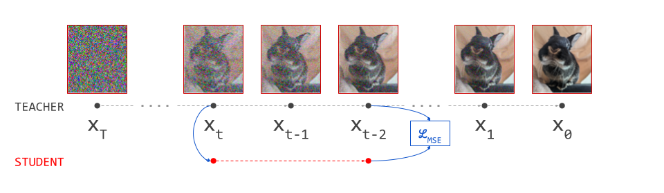
To reduce the number of sampling steps further, it can be applied repeatedly. In theory, one can go all the way down to single-step sampling by applying the procedure \(\log_2 N\) times. This addresses several shortcomings of the previous approach:

  • At each distillation stage, only two consecutive sampling steps are required, which is significantly cheaper than running the whole sampling procedure end-to-end. Therefore it can be done on-the-fly during training, and pre-generating the training dataset is no longer required.
  • The original training dataset used for the teacher model can be reused, if it is available (or any other dataset!). This helps to focus learning on the part of input space that is relevant and interesting.
  • While we could go all the way down to 1 step, the iterative nature of the procedure enables a trade-off between quality and compute cost. Going down to 4 or 8 steps turns out to help a lot to keep the inevitable quality loss from distillation at bay, while still speeding up sampling very significantly. This also provides a much better trade-off than simply reducing the number of sampling steps for the teacher model, instead of distilling it (see Figure 4 in the paper).

Aside: v-prediction

The most common parameterisation for training diffusion models in the image domain, where the neural network predicts the standardised Gaussian noise variable \(\varepsilon\), causes problems for progressive distillation. The implicit relative weighting of noise levels in the MSE loss w.r.t. \(\varepsilon\) is particularly suitable for visual data, because it maps well to the human visual system’s varying sensitivity to low and high spatial frequencies. This is why it is so commonly used.

To obtain a prediction in input space \(\hat{\mathbf{x}}_0\) from a model that predicts \(\varepsilon\) from the noisy input \(\mathbf{x}_t\), we can use the following formula:

\[\hat{\mathbf{x}}_0 = \alpha_t^{-1} \left( \mathbf{x}_t - \sigma_t \varepsilon (\mathbf{x}_t) \right) .\]

Here, \(\sigma_t\) represents the standard deviation of the noise at time step \(t\). (For variance-preserving diffusion, the scale factor \(\alpha_t = \sqrt{1 - \sigma_t^2}\), for variance-exploding diffusion, \(\alpha_t = 1\).)

At high noise levels, \(\mathbf{x}_t\) is dominated by noise, so the difference between \(\mathbf{x}_t\) and the scaled noise prediction is potentially quite small – but this difference entirely determines the prediction in input space \(\hat{\mathbf{x}}_0\)! This means any prediction errors may get amplified. In standard diffusion models, this is not a problem in practice, because errors can be corrected over many steps of sampling. In progressive distillation, this becomes a problem in later iterations, where we mainly evaluate the model at high noise levels (in the limit of a single-step model, the model is only ever evaluated at the highest noise level).

It turns out this issue can be addressed simply by parameterising the model to predict \(\mathbf{x}_0\) instead, but the progressive distillation paper also introduces a new prediction target \(\mathbf{v} = \alpha_t \varepsilon - \sigma_t \mathbf{x}_0\) (“velocity”, see section 4 and appendix D). This has some really nice properties, and has also become quite popular beyond just distillation applications in recent times.

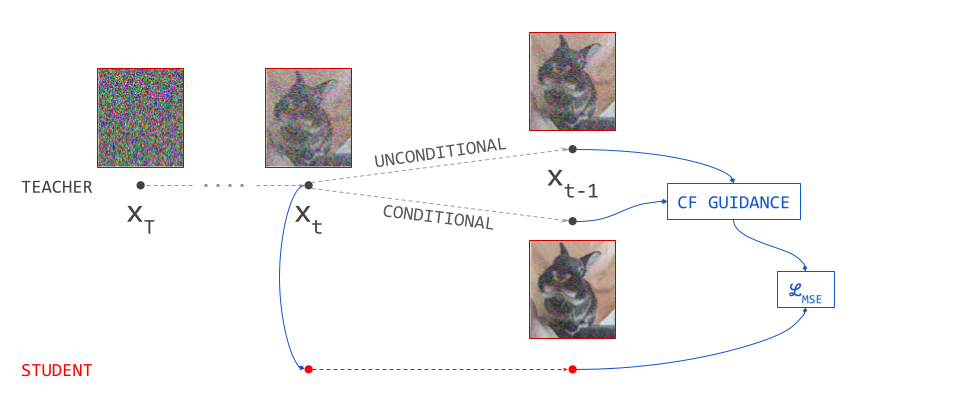
Guidance distillation

Before moving on to more advanced diffusion distillation methods that reduce the number of sampling steps, it’s worth looking at guidance distillation. The goal of this method is not to achieve high-quality samples in fewer steps, but rather to make each step computationally cheaper when using classifier-free guidance15. I have already dedicated two entire blog posts specifically to diffusion guidance, so I will not recap the concept here. Check them out first if you’re not familiar:

The use of classifier-free guidance requires two model evaluations per sampling step: one conditional, one unconditional. This makes sampling roughly twice as expensive, as the main cost is in the model evaluations. To avoid paying that cost, we can distill predictions that result from guidance into a model that predicts them directly in a single forward pass, conditioned on the chosen guidance scale16.

While guidance distillation does not reduce the number of sampling steps, it roughly halves the required computation per step, so it still makes sampling roughly twice as fast. It can also be combined with other forms of distillation. This is useful, because reducing the number of sampling steps actually reduces the impact of guidance, which relies on repeated small adjustments to update directions to work. Applying guidance distillation before another distillation method can help ensure that the original effect is preserved as the number of steps is reduced.

Diagram showing guidance distillation. A single step of sampling with classifier-free guidance (requiring two forward passes through the diffusion model) is distilled into a single forward pass.

Rectified flow

One way to understand the requirement for diffusion sampling to take many small steps, is through the lens of curvature: we can only take steps in a straight line, so if the steps we take are too large, we end up “falling off” the curve, leading to noticeable approximation errors.

As mentioned before, some sampling algorithms compensate for this by using curvature information to determine the step size, or by injecting noise to reduce error accumulation. The rectified flow method17 takes a more drastic approach: what if we just replace these curved paths between samples from the noise and data distributions with another set of paths that are significantly less curved?

This is possible using a procedure that resembles distillation, though it doesn’t quite have the same goal: whereas distillation tries to learn better/faster approximations of existing paths between samples from the noise and data distributions, the reflow procedure replaces the paths with a new set of paths altogether. We get a new model that gives rise to a set of paths with a lower cost in the “optimal transport” sense. Concretely, this means the paths are less curved. They will also typically connect different pairs of samples than before. In some sense, the mapping from noise to data is “rewired” to be more straight.

Diagram showing the old and new paths associated with data point x0 after applying the reflow procedure. The new path is significantly less curved (though not completely straight), and connects x0 to a different sample from the noise distribution than before.

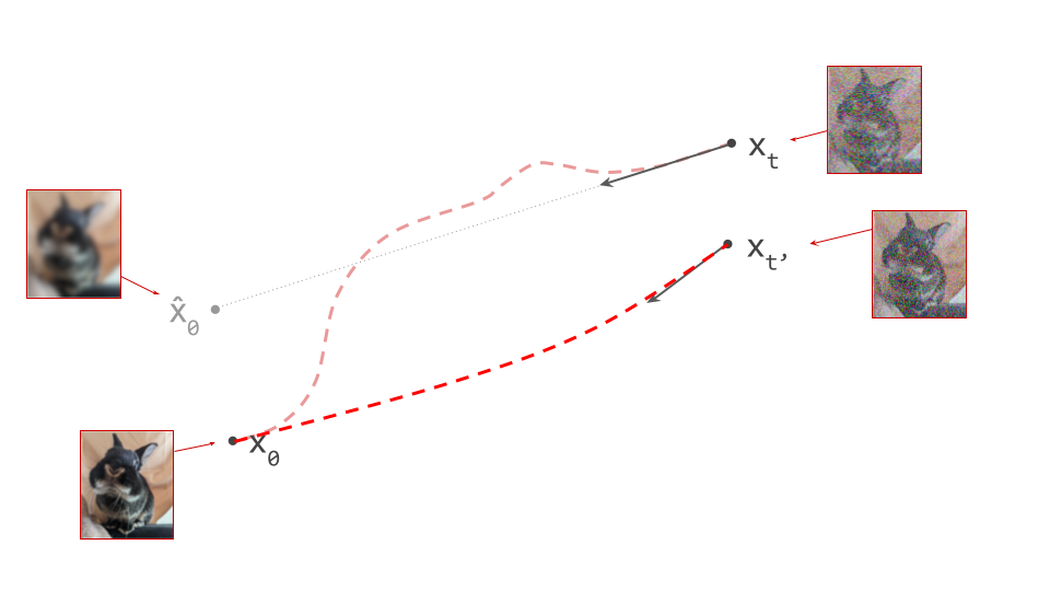
Lower curvature means we can take fewer, larger steps when sampling from this new model using our favourite sampling algorithm, while still keeping the approximation error at bay. But aside from that, this also greatly increases the efficacy of distillation, presumably because it makes the task easier.

The procedure can be applied recursively, to yield and even straighter set of paths. After an infinite number of applications, the paths should be completely straight. In practice, this only works up to a certain point, because each application of the procedure yields a new model which approximates the previous, so errors can quickly accumulate. Luckily, only one or two applications are needed to get paths that are mostly straight.

This method was successfully applied to a Stable Diffusion model18 and followed by a distillation step using a perceptual loss19. The resulting model produces reasonable samples in a single forward pass. One downside of the method is that each reflow step requires the generation of a dataset of sample pairs (data and corresponding noise) using a deterministic sampling algorithm, which usually needs to be done offline to be practical.

Consistency distillation & TRACT

As we covered before, diffusion sampling traces a curved path through input space, and at each point on this curve, the diffusion model predicts the tangent direction. What if we had a model that could predict the endpoint of the path on the side of the data distribution instead, allowing us to jump there from anywhere on the path in one step? Then the degree of curvature simply wouldn’t matter.

This is what consistency models20 do. They look very similar to diffusion models, but they predict a different kind of quantity: an endpoint of the path, rather than a tangent direction. In a sense, diffusion models and consistency models are just two different ways to describe a mapping between noise and data. Perhaps it could be useful to think of consistency models as the “integral form” of diffusion models (or, equivalently, of diffusion models as the “derivative form” of consistency models).

Diagram showing the difference between the predictions from a diffusion model (grey) and a consistency model (blue). The former predicts a tangent direction to the path, the latter predicts the endpoint of the path on the data side.

While it is possible to train a consistency model from scratch (though not that straightforward, in my opinion – more on this later), a more practical route to obtaining a consistency model is to train a diffusion model first, and then distill it. This process is called consistency distillation.

It’s worth noting that the resulting model looks quite similar to what we get when distilling the diffusion sampling procedure into a single forward pass. However, that only lets us jump from one endpoint of a path (at the noise side) to the other (at the data side). Consistency models are able to jump to the endpoint on the data side from anywhere on the path.

Learning to map any point on a path to its endpoint requires paired data, so it would seem that we once again need to run the full sampling process to obtain training targets from the teacher model, which is expensive. However, this can be avoided using a bootstrapping mechanism where, in addition to learning from the teacher, the student also learns from itself.

This hinges on the following principle: the prediction of the consistency model along all points on the path should be the same. Therefore, if we take a step along the path using the teacher, the student’s prediction should be unchanged. Let \(f(\mathbf{x}_t, t)\) represent the student (a consistency model), then we have:

\[f(\mathbf{x}_{t - \Delta t}, t - \Delta t) \equiv f(\mathbf{x}_t, t),\]

where \(\Delta t\) is the step size and \(\mathbf{x}_{t - \Delta t}\) is the result of a sampling step starting from \(\mathbf{x}_t\), with the update direction given by the teacher. The prediction remains consistent along all points on the path, which is where the name comes from. Note that this is not at all true for diffusion models.

Concurrently with the consistency models paper, transitive closure time-distillation (TRACT)21 was proposed as an improvement over progressive distilation, using a very similar bootstrapping mechanism. The details of implementation differ, and rather than predicting the endpoint of a path from any point on the path, as consistency models do, TRACT instead divides the range of time steps into intervals, with the distilled model predicting points on paths at the boundaries of those intervals.

Diagram showing how TRACT divides the time step range into intervals. From any point on the path, the student is trained to predict the point corresponding to the left boundary of the interval the current point is in. This is the same target as for consistency models, but applied separately to non-overlapping segments of the path, rather than to the path as a whole.

Like progressive distillation, this is a procedure that can be repeated with fewer and fewer intervals, to eventually end up with something that looks pretty much the same as a consistency model (when using a single interval that encompasses the entire time step range). TRACT was proposed as an alternative to progressive distillation which requires fewer distillation stages, thus reducing the potential for error accumulation.

It is well-known that diffusion models benefit significantly from weight averaging22 23, so both TRACT and the original formulation of consistency models use an exponential moving average (EMA) of the student’s weights to construct a self-teacher model, which effectively acts as an additional teacher in the distillation process, alongside the diffusion model. That said, a more recent iteration of consistency models24 does not use EMA.

Another strategy to improve consistency models is to use alternative loss functions for distillation, such as a perceptual loss like LPIPS19, instead of the usual mean squared error (MSE), which we’ve also seen used before with rectified flow17.

Recent work on distilling a Stable Diffusion model into a latent consistency model25 has yielded compelling results, producing high-resolution images in 1 to 4 sampling steps.

Consistency trajectory models26 are a generalisation of both diffusion models and consistency models, enabling prediction of any point along a path from any other point before it, as well as tangent directions. To achieve this, they are conditioned on two time steps, indicating the start and end positions. When both time steps are the same, the model predicts the tangent direction, like a diffusion model would.

BOOT: data-free distillation

Instead of predicting the endpoint of a path at the data side from any point on that path, as consistency models learn to do, we can try to predict any point on the path from its endpoint at the noise side. This is what BOOT27 does, providing yet another way to describe a mapping between noise and data. Comparing this formulation to consistency models, one looks like the “transpose” of the other (see diagram below). For those of you who remember word2vec28, it reminds me lot of the relationship between the skip-gram and continuous bag-of-words (CBoW) methods!

Diagram showing the inputs and prediction targets for the student in consistency distillation (top) and BOOT (bottom), based on Figure 2 in Gu et al. 2023.

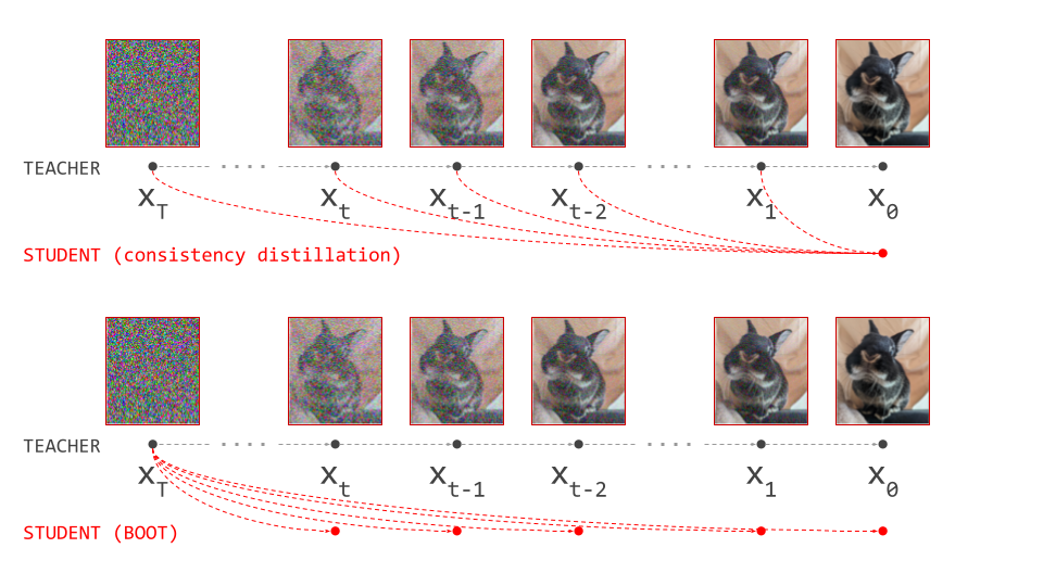
Just like consistency models, this formulation enables a form of bootstrapping to avoid having to run the full sampling procedure using the teacher (hence the name, I presume): predict \(\mathbf{x}_t = f(\varepsilon, t)\) using the student, run a teacher sampling step to obtain \(\mathbf{x}_{t - \Delta t}\), then train the student so that \(f(\varepsilon, t - \Delta t) \equiv \mathbf{x}_{t - \Delta t}\).

Because the student only ever takes the noise \(\varepsilon\) as input, we do not need any training data to perform distillation. This is also the case when we directly distill the diffusion sampling procedure into a single forward pass – though of course in that case, we can’t avoid running the full sampling procedure using the teacher.

There is one big caveat however: it turns out that predicting \(\mathbf{x}_t\) is actually quite hard to learn. But there is a neat workaround for this: instead of predicting \(\mathbf{x}_t\) directly, we first convert it into a different target using the identity \(\mathbf{x}_t = \alpha_t \mathbf{x}_0 + \sigma_t \varepsilon\). Since \(\varepsilon\) is given, we can rewrite this as \(\mathbf{x}_0 = \frac{\mathbf{x}_t - \sigma_t \varepsilon}{\alpha_t}\), which corresponds to an estimate of the clean input. Whereas \(\mathbf{x}_t\) looks like a noisy image, this single-step \(\mathbf{x}_0\) estimate looks like a blurry image instead, lacking high-frequency content. This is a lot easier for a neural network to predict.

If we see \(\mathbf{x}_t\) as a mixture of signal and noise, we are basically extracting the “signal” component and predicting that instead. We can easily convert such a prediction back to a prediction of \(\mathbf{x}_t\) using the same formula. Just like \(\mathbf{x}_t\) traces a path through input space which can be described by an ODE, this time-dependent \(\mathbf{x}_0\)-estimate does as well. The BOOT authors call the ODE describing this path the signal-ODE.

Unlike in the original consistency models formulation (as well as TRACT), no exponential moving average is used for the bootstrapping procedure. To reduce error accumulation, the authors suggest using a higher-order solver to run the teacher sampling step. Another requirement to make this method work well is an auxiliary “boundary loss”, ensuring the distilled model is well-behaved at \(t = T\) (i.e. at the highest noise level).

Sampling with neural operators

Diffusion sampling with neural operators (DSNO; also known as DFNO, the acronym seems to have changed at some point!)29 works by training a model that can predict an entire path from noise to data given a noise sample in a single forward pass. While the inputs (\(\varepsilon\)) and targets (\(\mathbf{x}_t\) at various \(t\)) are the same as for a BOOT-distilled student model, the latter is only able to produce a single point on the path at a time.

This seems ambitious – how can a neural network predict an entire path at once, from noise all the way to data? The so-called Fourier neural operator (FNO)30 is used to achieve this. By imposing certain architectural constraints, adding temporal convolution layers and making use of the Fourier transform to represent functions of time in frequency space, we obtain a model that can produce predictions for any number of time steps at once.

A natural question is then: why would we actually want to predict the entire path? When sampling, we only really care about the final outcome, i.e. the endpoint of the path at the data side (\(t = 0\)). For BOOT, the point of predicting the other points on the path is to enable the bootstrapping mechanism used for training. But DSNO does not involve any bootstrapping, so what is the point of doing this here?

The answer probably lies in the inductive bias of the temporal convolution layers, combined with the relative smoothness of the paths through input space learnt by diffusion models. Thanks to this architectural prior, training on other points on the path also helps to improve the quality of the predictions at the endpoint on the data side, that is, the only point on the path we actually care about when sampling in a single step. I have to admit I am not 100% confident that this is the only reason – if there is another compelling reason why this works, please let me know!

Score distillation sampling

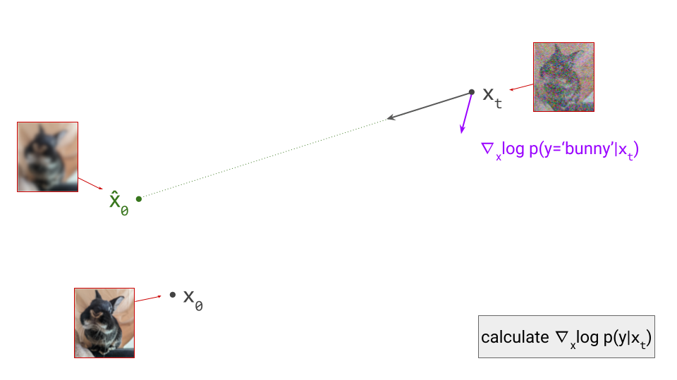
Score distillation sampling (SDS)31 is a bit different from the methods we’ve discussed so far: rather than accelerating sampling by producing a student model that needs fewer steps for high-quality output, this method is aimed at optimisation of parameterised representations of images. This means that it enables diffusion models to operate on other representations of images than pixel grids, even though that is what they were trained on – as long as those representations produce pixel space outputs that are differentiable w.r.t. their parameters32.

As a concrete example of this, SDS was actually introduced to enable text-to-3D. This is achieved through optimisation of Neural Radiance Field (NeRF)33 representations of 3D models, using a pretrained image diffusion model applied to random 2D projections to control the generated 3D models through text prompts (DreamFusion).

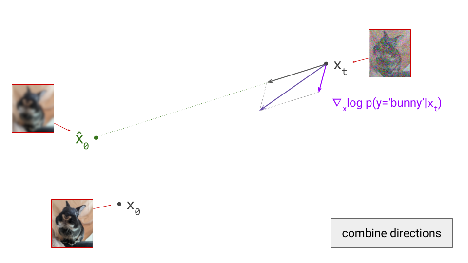
Naively, one could think that simply backpropagating the diffusion loss at various time steps through the pixel space output produced by the parameterised representation should do the trick. This yields gradient updates w.r.t. the representation parameters that minimise the diffusion loss, which should make the pixel space output look more like a plausible image. Unfortunately, this method doesn’t work very well, even when applied directly to pixel representations.

It turns out this is primarily caused by a particular factor in the gradient, which corresponds to the Jacobian of the diffusion model itself. This Jacobian is poorly conditioned for low noise levels. Simply omitting this factor altogether (i.e. replacing it with the identity matrix) makes things work much better. As an added bonus, it means we can avoid having to backpropagate through the diffusion model. All we need is forward passes, just like in regular diffusion sampling algorithms!

After modifying the gradient in a fairly ad-hoc fashion, it’s worth asking what loss function this modified gradient corresponds to. This is actually the same loss function used in probability density distillation34, which was originally developed to distill autoregressive models for audio waveform generation into feedforward models. I won’t elaborate on this connection here, except to mention that it provides an explanation for the mode-seeking behaviour that SDS seems to exhibit. This behaviour often results in pathologies, which require additional regularisation loss terms to mitigate. It was also found that using a high guidance scale for the teacher (a higher value than one would normally use to sample images) helps to improve results.

Noise-free score distillation (NFSD)35 is a variant that modifies the gradient further to enable the use of lower guidance scales, which results in better sample quality and diversity. Variational score distillation sampling (VSD)36 improves over SDS by optimising a distribution over parameterised representations, rather than a point estimate, which also eliminates the need for high guidance scales.

VSD has in turn been used as a component in more traditional diffusion distillation strategies, aimed at reducing the number of sampling steps. A single-step image generator can easily be reinterpreted as a distribution over parameterised representations, which makes VSD readily applicable to this setting, even if it was originally conceived to improve text-to-3D rather than speed up image generation.

Diff-Instruct37 can be seen as such an application, although it was actually published concurrently with VSD. To distill the knowledge from a diffusion model into a single-step feed-forward generator, they suggest minimising the integral KL divergence (IKL), which is a weighted integral of the KL divergence along the diffusion process (w.r.t. time). Its gradient is estimated by contrasting the predictions of the teacher and those of an auxiliary diffusion model which is concurrently trained on generator outputs. This concurrent training gives it a bit of a GAN38 flavour, but note that the generator and the auxiliary model are not adversaries in this case. As with SDS, the gradient of the IKL with respect to the generator parameters only requires evaluating the diffusion model teacher, but not backpropagating through it – though training the auxiliary diffusion model on generator outputs does of course require backpropagation.

Distribution matching distillation (DMD)39 arrives at a very similar formulation from a different angle. Just like in Diff-Instruct, a concurrently trained diffusion model of the generator outputs is used, and its predictions are contrasted against those of the teacher to obtain gradients for the feed-forward generator. This is combined with a perceptual regression loss (LPIPS19) on paired data from the teacher, which is pre-generated offline. The latter is only applied on a small subset of training examples, making the computational cost of this pre-generation step less prohibitive.

Adversarial distillation

Before diffusion models completely took over in the space of image generation, generative adversarial networks (GANs)38 offered the best visual fidelity, at the cost of mode-dropping: the diversity of model outputs usually does not reflect the diversity of the training data, but at least they look good. In other words, they trade off diversity for quality. On top of that, GANs generate images in a single forward pass, so they are very fast – much faster than diffusion model sampling.

It is therefore unsurprising that some works have sought to combine the benefits of adversarial models and diffusion models. There are many ways to do so: denoising diffusion GANs40 and adversarial score matching41 are just two examples.

A more recent example is UFOGen42, which proposes an adversarial finetuning approach for diffusion models that looks a lot like distillation, but actually isn’t distillation, in the strict sense of the word. UFOGen combines the standard diffusion loss with an adversarial loss. Whereas the standard diffusion loss by itself would result in a model that tries to predict the conditional expectation \(\mathbb{E}\left[\mathbf{x}_0 \mid \mathbf{x}_t \right]\), the additional adversarial loss term allows the model to deviate from this and produce less blurry predictions at high noise levels. The result is a reduction in diversity, but it also enables faster sampling. Both the generator and the discriminator are initialised from the parameters of a pre-trained diffusion model, but this pre-trained model is not evaluated to produce training targets, as would be the case in a distillation approach. Nevertheless, it merits inclusion here, as it is intended to achieve the same goal as most of the distillation approaches that we’ve discussed.

Adversarial diffusion distillation43, on the other hand, is a “true” distillation approach, combining score distillation sampling (SDS) with an adversarial loss. It makes use of a discriminator built on top of features from an image representation learning model, DINO44, which was previously also used for a purely adversarial text-to-image model, StyleGAN-T45. The resulting student model enables single-step sampling, but can also be sampled from with multiple steps to improve the quality of the results. This method was used for SDXL Turbo, a text-to-image system that enables realtime generation – the generated image is updated as you type.

But what about “no free lunch”?

Why is it that we can get these distilled models to produce compelling samples in just a few steps, when diffusion models take tens or hundreds of steps to achieve the same thing? What about “no such thing as a free lunch”?

At first glance, diffusion distillation certainly seems like a counterexample to what is widely considered a universal truth in machine learning, but there is more to it. Up to a point, diffusion model sampling can probably be made more efficient through distillation at no noticeable cost to model quality, but the regime targeted by most distillation methods (i.e. 1-4 sampling steps) goes far beyond that point, and trades off quality for speed. Distillation is almost always “lossy” in practice, and the student cannot be expected to perfectly mimic the teacher’s predictions. This results in errors which can accumulate across sampling steps, or for some methods, across different phases of the distillation process.

What does this trade-off look like? That depends on the distillation method. For most methods, the decrease in model quality directly affects the perceptual quality of the output: samples from distilled models can often look blurry, or the fine-grained details might look sharp but less realistic, which is especially noticeable in images of human faces. The use of adversarial losses based on discriminators, or perceptual loss functions such as LPIPS19, is intended to mitigate some of this degradation, by further focusing model capacity on signal content that is perceptually relevant.

Some methods preserve output quality and fidelity of high-frequency content to a remarkable degree, but this then usually comes at cost to the diversity of the samples instead. The adversarial methods discussed earlier are a great example of this, as well as methods based on score distillation sampling, which implicitly optimise a mode-seeking loss function.

So if distillation implies a loss of model quality, is training a diffusion model and then distilling it even worthwhile? Why not train a different type of model instead, such as a GAN, which produces a single-step generator out of the box, without requiring distillation? The key here is that distillation provides us with some degree of control over this trade-off. We gain flexibility: we get to choose how many steps we can afford, and by choosing the right method, we can decide exactly how we’re going to cut corners. Do we care more about fidelity or diversity? It’s our choice!

Do we really need a teacher?

Once we have established that diffusion distillation gives us the kind of model that we are after, with the right trade-offs in terms of output quality, diversity and sampling speed, it’s worth asking whether we even needed distillation to arrive at this model to begin with. In a sense, once we’ve obtained a particular model through distillation, that’s an existence proof, showing that such a model is feasible in practice – but it does not prove that we arrived at that model in the most efficient way possible. Perhaps there is a shorter route? Could we train such a model from scratch, and skip the training of the teacher model entirely?

The answer depends on the distillation method. For certain types of models that can be obtained through diffusion distillation, there are indeed alternative training recipes that do not require distillation at all. However, these tend not to work quite as well as the distillation route. Perhaps this is not that surprising: it has long been known that when distilling a large neural network into a smaller one, we can often get better results than when we train that smaller network from scratch11. The same phenomenon is at play here, because we are distilling a sampling procedure with many steps into one with considerably fewer steps. If we look at the computational graphs of these sampling procedures, the former is much “deeper” than the latter, so what we’re doing looks very similar to distilling a large model into a smaller one.

One instance where you have the choice of distillation or training from scratch, is consistency models. The paper that introduced them20 describes both consistency distillation and consistency training. The latter requires a few tricks to work well, including schedules for some of the hyperparameters to create a kind of “curriculum”, so it is arguably a bit more involved than diffusion model training.

Charting the maze between data and noise

One interesting perspective on diffusion model training that is particularly relevant to distillation, is that it provides a way to uncover an optimal transport map between distributions46. Through the probability flow ODE formulation2, we can see that diffusion models learn a bijection between noise and data, and it turns out that this mapping is approximately optimal in some sense.

This also explains the observation that different diffusion models trained on similar data tend to learn similar mappings: they are all trying to approximate the same optimum! I tweeted (X’ed?) about this a while back:

So far, it seems that diffusion model training is the simplest and most effective (i.e. scalable) way we know of to approximate this optimal mapping, but it is not the only way: consistency training represents a compelling alternative strategy. This makes me wonder what other approaches are yet to be discovered, and whether we might be able to find methods that are even simpler than diffusion model training, or more statistically efficient.

Another interesting link between some of these methods can be found by looking more closely at curvature. The paths connecting samples from the noise and data distributions uncovered by diffusion model training tend to be curved. This is why we need many discrete steps to approximate them accurately when sampling.

We discussed a few approaches to sidestep this issue: consistency models20 21 avoid it by changing the prediction target of the model, from the tangent direction at the current position to the endpoint of the curve at the data side. Rectified flow17 instead replaces the curved paths altogether, with a set of paths that are much straighter. But for perfectly straight paths, the tangent direction will actually point to the endpoint! In other words: in the limiting case of perfectly straight paths, consistency models and diffusion models predict the same thing, and become indistinguishable from each other.

Is that observation practically relevant? Probably not – it’s just a neat connection. But I think it’s worthwhile to cultivate a deeper understanding of deterministic mappings between distributions and how to uncover them at scale, as well as the different ways to parameterise them and represent them. I think this is fertile ground for innovations in diffusion distillation, as well as generative modelling through iterative refinement in a broader sense.

Closing thoughts

As I mentioned at the beginning, this was supposed to be a fairly high-level treatment of diffusion distillation, and why there are so many different ways to do it. I ended up doing a bit of a deep dive, because it’s difficult to talk about the connections between all these methods without also explaining the methods themselves. In reading up on the subject and trying to explain things concisely, I actually learnt a lot. If you want to learn about a particular subject in machine learning research (or really anything else), I can heartily recommend writing a blog post about it.

To wrap things up, I wanted to take a step back and identify a few patterns and trends. Although there is a huge variety of diffusion distillation methods, there are clearly some common tricks and ideas that come back frequently:

  • Using deterministic sampling algorithms to obtain targets from the teacher is something that almost all methods rely on. DDIM4 is popular, but more advanced methods (e.g. higher-order methods) are also an option.
  • The parameters of the student network are usually initialised from those of the teacher. This doesn’t just accelerate convergence, for some methods this is essential for them to work at all. We can do this because the architectures of the teacher and student are often identical, unlike in distillation of discriminative models.
  • Several methods make use of perceptual losses such as LPIPS19 to reduce the negative impact of distillation on low-level perceptual quality.
  • Bootstrapping, i.e. having the student learn from itself, is a useful trick to avoid having to run the full sampling algorithm to obtain targets from the teacher. Sometimes using the exponential moving average of the student’s parameters is found to help for this, but this isn’t as clear-cut.

Distillation can interact with other modelling choices. One important example is classifier-free guidance15, which implicitly relies on there being many sampling steps. Guidance operates by modifying the direction in input space predicted by the diffusion model, and the effect of this will inevitably be reduced if only a few sampling steps are taken. For some methods, applying guidance after distillation doesn’t actually make sense anymore, because the student no longer predicts a direction in input space. Luckily guidance distillation16 can be used to mitigate the impact of this.

Another instance of this is latent diffusion47: when applying distillation to a diffusion model trained in latent space, one important question to address is whether the loss should be applied to the latent representation or to pixels. As an example, the adversarial diffusion distillation (ADD) paper43 explicitly suggests calculating the distillation loss in pixel space for improved stability.

The procedure of first solving a problem as well as possible, and then looking for shortcuts that yield acceptable trade-offs, is very effective in machine learning in general. Diffusion distillation is a quintessential example of this. There is still no such thing as a free lunch, but diffusion distillation enables us to cut corners with intention, and that’s worth a lot!

If you would like to cite this post in an academic context, you can use this BibTeX snippet:

@misc{dieleman2024distillation,
  author = {Dieleman, Sander},
  title = {The paradox of diffusion distillation},
  url = {https://sander.ai/2024/02/28/paradox.html},
  year = {2024}
}

Acknowledgements

Thanks once again to Bundle the bunny for modelling, and to kipply for permission to use this photograph. Thanks to Emiel Hoogeboom, Valentin De Bortoli, Pierre Richemond, Andriy Mnih and all my colleagues at Google DeepMind for various discussions, which continue to shape my thoughts on diffusion models and beyond!

References

  1. Ho, Jain, Abbeel, “Denoising Diffusion Probabilistic Models”, 2020.  2

  2. Song, Sohl-Dickstein, Kingma, Kumar, Ermon and Poole, “Score-Based Generative Modeling through Stochastic Differential Equations”, International Conference on Learning Representations, 2021.  2 3

  3. Karras, Aittala, Aila, Laine, “Elucidating the Design Space of Diffusion-Based Generative Models”, Neural Information Processing Systems, 2022.  2 3

  4. Song, Meng, Ermon, “Denoising Diffusion Implicit Models”, International Conference on Learning Representations, 2021.  2 3

  5. Jolicoeur-Martineau, Li, Piché-Taillefer, Kachman, Mitliagkas, “Gotta Go Fast When Generating Data with Score-Based Models”, arXiv, 2021. 

  6. Dockhorn, Vahdat, Kreis, “GENIE: Higher-Order Denoising Diffusion Solvers”, Neural Information Processing Systems, 2022. 

  7. Liu, Ren, Lin, Zhao, “Pseudo Numerical Methods for Diffusion Models on Manifolds”, International Conference on Learning Representations, 2022. 

  8. Zhang, Chen, “Fast Sampling of Diffusion Models with Exponential Integrator”, International Conference on Learning Representations, 2023. 

  9. Lu, Zhou, Bao, Chen, Li, Zhu, “DPM-Solver: A Fast ODE Solver for Diffusion Probabilistic Model Sampling in Around 10 Steps”, Neural Information Processing Systems, 2022. 

  10. Lu, Zhou, Bao, Chen, Li, Zhu, “DPM-Solver++: Fast Solver for Guided Sampling of Diffusion Probabilistic Models”, arXiv, 2022. 

  11. Hinton, Vinyals, Dean, “Distilling the Knowledge in a Neural Network”, NeurIPS Deep Learning Workshop, 2014.  2

  12. Luo, “A Comprehensive Survey on Knowledge Distillation of Diffusion Models”, arXiv, 2023. 

  13. Luhman, Luhman, “Knowledge Distillation in Iterative Generative Models for Improved Sampling Speed”, arXiv, 2021. 

  14. Salimans, Ho, “Progressive Distillation for Fast Sampling of Diffusion Models”, International Conference on Learning Representations, 2022. 

  15. Ho, Salimans, “Classifier-Free Diffusion Guidance”, Neural Information Processing Systems, 2021.  2

  16. Meng, Rombach, Gao, Kingma, Ermon, Ho, Salimans, “On Distillation of Guided Diffusion Models”, Computer Vision and Pattern Recognition, 2023.  2

  17. Liu, Gong, Liu, “Flow Straight and Fast: Learning to Generate and Transfer Data with Rectified Flow”, International Conference on Learning Representations, 2023.  2 3

  18. Liu, Zhang, Ma, Peng, Liu, “InstaFlow: One Step is Enough for High-Quality Diffusion-Based Text-to-Image Generation”, arXiv, 2023. 

  19. Zhang, Isola, Efros, Shechtman, Wang, “The Unreasonable Effectiveness of Deep Features as a Perceptual Metric”, Computer Vision and Pattern Recognition, 2018.  2 3 4 5

  20. Song, Dhariwal, Chen, Sutskever, “Consistency Models”, International Conference on Machine Learning, 2023.  2 3

  21. Berthelot, Autef, Lin, Yap, Zhai, Hu, Zheng, Talbott, Gu, “TRACT: Denoising Diffusion Models with Transitive Closure Time-Distillation”, arXiv, 2023.  2

  22. Song, Ermon, “Improved Techniques for Training Score-Based Generative Models”, Neural Information Processing Systems, 2020. 

  23. Karras, Aittala, Lehtinen, Hellsten, Aila, Laine, “Analyzing and Improving the Training Dynamics of Diffusion Models”, arXiv, 2023. 

  24. Song, Dhariwal, “Improved Techniques for Training Consistency Models”, International Conference on Learnign Representations, 2024. 

  25. Luo,Tan, Huang, Li, Zhao, “Latent Consistency Models: Synthesizing High-Resolution Images with Few-Step Inference”, arXiv, 2023. 

  26. Kim, Lai, Liao, Murata, Takida, Uesaka, He, Mitsufuji, Ermon, “Consistency Trajectory Models: Learning Probability Flow ODE Trajectory of Diffusion”, International Conference on Learning Representations, 2024. 

  27. Gu, Zhai, Zhang, Liu, Susskind, “BOOT: Data-free Distillation of Denoising Diffusion Models with Bootstrapping”, arXiv, 2023. 

  28. Mikolov, Chen, Corrado, Dean, “Efficient Estimation of Word Representations in Vector Space”, International Conference on Learning Representation, 2013. 

  29. Zheng, Nie, Vahdat, Azizzadenesheli, Anandkumar, “Fast Sampling of Diffusion Models via Operator Learning”, International Conference on Machine Learning, 2023. 

  30. Li, Kovachki, Azizzadenesheli, Liu, Bhattacharya, Stuart, Anandkumar, “Fourier neural operator for parametric partial differential equations”, International Conference on Learning Representations, 2021. 

  31. Poole, Jain, Barron, Mildenhall, “DreamFusion: Text-to-3D using 2D Diffusion”, arXiv, 2022. 

  32. Mordvintsev, Pezzotti, Schubert, Olah, “Differentiable Image Parameterizations”, Distill, 2018. 

  33. Mildenhall, Srinivasan, Tancik, Barron, Ramamoorthi, Ng, “NeRF: Representing Scenes as Neural Radiance Fields for View Synthesis”, European Conference on Computer Vision, 2020. 

  34. Van den Oord, Li, Babuschkin, Simonyan, Vinyals, Kavukcuoglu, van den Driessche, Lockhart, Cobo, Stimberg, Casagrande, Grewe, Noury, Dieleman, Elsen, Kalchbrenner, Zen, Graves, King, Walters, Belov and Hassabis, “Parallel WaveNet: Fast High-Fidelity Speech Synthesis”, International Conference on Machine Learning, 2018. 

  35. Katzir, Patashnik, Cohen-Or, Lischinski, “Noise-free Score Distillation”, International Conference on Learning Representations, 2024. 

  36. Wang, Lu, Wang, Bao, Li, Su, Zhu, “ProlificDreamer: High-Fidelity and Diverse Text-to-3D Generation with Variational Score Distillation”, Neural Information Processing Systems, 2023. 

  37. Luo, Hu, Zhang, Sun, Li, Zhang, “Diff-Instruct: A Universal Approach for Transferring Knowledge From Pre-trained Diffusion Models”, Neural Information Processing Systems, 2023. 

  38. Goodfellow, Pouget-Abadie, Mirza, Xu, Warde-Farley, Ozair, Courville and Bengio, “Generative Adversarial Nets”, Neural Information Processing Systems, 2014.  2

  39. Yin, Gharbi, Zhang, Shechtman, Durand, Freeman, Park, “One-step Diffusion with Distribution Matching Distillation”, arXiv, 2023. 

  40. Xiao, Kreis, Vahdat, “Tackling the Generative Learning Trilemma with Denoising Diffusion GANs”, International Conference on Learning Representations, 2022. 

  41. Jolicoeur-Martineau, Piché-Taillefer, Tachet des Combes, Mitliagkas, “Adversarial score matching and improved sampling for image generation”, International Conference on Learning Representations, 2021. 

  42. Xu, Zhao, Xiao, Hou, “UFOGen: You Forward Once Large Scale Text-to-Image Generation via Diffusion GANs”, arXiv, 2023. 

  43. Sauer, Lorenz, Blattmann, Rombach, “Adversarial Diffusion Distillation”, arXiv, 2023.  2

  44. Caron, Touvron, Misra, Jégou, Mairal, Bojanowski, Joulin, “Emerging Properties in Self-Supervised Vision Transformers”, International Conference on Computer Vision, 2021. 

  45. Sauer, Karras, Laine, Geiger, Aila, “StyleGAN-T: Unlocking the Power of GANs for Fast Large-Scale Text-to-Image Synthesis”, International Conference on Machine Learning, 2023. 

  46. Khrulkov, Ryzhakov, Chertkov, Oseledets, “Understanding DDPM Latent Codes Through Optimal Transport”, International Conference on Learning Representations, 2023. 

  47. Rombach, Blattmann, Lorenz, Esser, Ommer, “High-Resolution Image Synthesis with Latent Diffusion Models”, Computer Vision and Pattern Recognition, 2022. 

The geometry of diffusion guidance

Guidance is a powerful method that can be used to enhance diffusion model sampling. As I’ve discussed in an earlier blog post, it’s almost like a cheat code: it can improve sample quality so much that it’s as if the model had ten times the number of parameters – an order of magnitude improvement, basically for free! This follow-up post provides a geometric interpretation and visualisation of the diffusion sampling procedure, which I’ve found particularly useful to explain how guidance works.

A word of warning about high-dimensional spaces

Sampling algorithms for diffusion models typically start by initialising a canvas with random noise, and then repeatedly updating this canvas based on model predictions, until a sample from the model distribution eventually emerges.

We will represent this canvas by a vector \(\mathbf{x}_t\), where \(t\) represents the current time step in the sampling procedure. By convention, the diffusion process which gradually corrupts inputs into random noise moves forward in time from \(t=0\) to \(t=T\), so the sampling procedure goes backward in time, from \(t=T\) to \(t=0\). Therefore \(\mathbf{x}_T\) corresponds to random noise, and \(\mathbf{x}_0\) corresponds to a sample from the data distribution.

\(\mathbf{x}_t\) is a high-dimensional vector: for example, if a diffusion model produces images of size 64x64, there are 12,288 different scalar intensity values (3 colour channels per pixel). The sampling procedure then traces a path through a 12,288-dimensional Euclidean space.

It’s pretty difficult for the human brain to comprehend what that actually looks like in practice. Because our intuition is firmly rooted in our 3D surroundings, it actually tends to fail us in surprising ways in high-dimensional spaces. A while back, I wrote a blog post about some of the implications for high-dimensional probability distributions in particular. This note about why high-dimensional spheres are “spikey” is also worth a read, if you quickly want to get a feel for how weird things can get. A more thorough treatment of high-dimensional geometry can be found in chapter 2 of ‘Foundations of Data Science’1 by Blum, Hopcroft and Kannan, which is available to download in PDF format.

Nevertheless, in this blog post, I will use diagrams that represent \(\mathbf{x}_t\) in two dimensions, because unfortunately that’s all the spatial dimensions available on your screen. This is dangerous: following our intuition in 2D might lead us to the wrong conclusions. But I’m going to do it anyway, because in spite of this, I’ve found these diagrams quite helpful to explain how manipulations such as guidance affect diffusion sampling in practice.

Here’s some advice from Geoff Hinton on dealing with high-dimensional spaces that may or may not help:

… anyway, you’ve been warned!

Visualising diffusion sampling

To start off, let’s visualise what a step of diffusion sampling typically looks like. I will use a real photograph to which I’ve added varying amounts of noise to stand in for intermediate samples in the diffusion sampling process:

Bundle the bunny, with varying amounts of noise added.
Bundle the bunny, with varying amounts of noise added. Photo credit: kipply.

During diffusion model training, examples of noisy images are produced by taking examples of clean images from the data distribution, and adding varying amounts of noise to them. This is what I’ve done above. During sampling, we start from a canvas that is pure noise, and then the model gradually removes random noise and replaces it with meaningful structure in accordance with the data distribution. Note that I will be using this set of images to represent intermediate samples from a model, even though that’s not how they were constructed. If the model is good enough, you shouldn’t be able to tell the difference anyway!

In the diagram below, we have an intermediate noisy sample \(\mathbf{x}_t\), somewhere in the middle of the sampling process, as well as the final output of that process \(\mathbf{x}_0\), which is noise-free:

Diagram showing an intermediate noisy sample, as well as the final output of the sampling process.

Imagine the two spatial dimensions of your screen representing just two of many thousands of pixel colour intensities (red, green or blue). Different spatial positions in the diagram correspond to different images. A single step in the sampling procedure is taken by using the model to predict where the final sample will end up. We’ll call this prediction \(\hat{\mathbf{x}}_0\):

Diagram showing the prediction of the final sample from the current step in the sampling process.

Note how this prediction is roughly in the direction of \(\mathbf{x}_0\), but we’re not able to predict \(\mathbf{x}_0\) exactly from the current point in the sampling process, \(\mathbf{x}_t\), because the noise obscures a lot of information (especially fine-grained details), which we aren’t able to fill in all in one go. Indeed, if we were, there would be no point to this iterative sampling procedure: we could just go directly from pure noise \(\mathbf{x}_T\) to a clean image \(\mathbf{x}_0\) in one step. (As an aside, this is more or less what Consistency Models2 try to achieve.)

Diffusion models estimate the expectation of \(\mathbf{x}_0\), given the current noisy input \(\mathbf{x}_t\): \(\hat{\mathbf{x}}_0 = \mathbb{E}[\mathbf{x}_0 \mid \mathbf{x}_t]\). At the highest noise levels, this expectation basically corresponds to the mean of the entire dataset, because very noisy inputs are not very informative. As a result, the prediction \(\hat{\mathbf{x}}_0\) will look like a very blurry image when visualised. At lower noise levels, this prediction will become sharper and sharper, and it will eventually resemble a sample from the data distribution. In a previous blog post, I go into a little bit more detail about why diffusion models end up estimating expectations.

In practice, diffusion models are often parameterised to predict noise, rather than clean input, which I also discussed in the same blog post. Some models also predict time-dependent linear combinations of the two. Long story short, all of these parameterisations are equivalent once the model has been trained, because a prediction of one of these quantities can be turned into a prediction of another through a linear combination of the prediction itself and the noisy input \(\mathbf{x}_t\). That’s why we can always get a prediction \(\hat{\mathbf{x}}_0\) out of any diffusion model, regardless of how it was parameterised or trained: for example, if the model predicts the noise, simply take the noisy input and subtract the predicted noise.

Diffusion model predictions also correspond to an estimate of the so-called score function, \(\nabla_{\mathbf{x}_t} \log p(\mathbf{x}_t)\). This can be interpreted as the direction in input space along which the log-likelihood of the input increases maximally. In other words, it’s the answer to the question: “how should I change the input to make it more likely?” Diffusion sampling now proceeds by taking a small step in the direction of this prediction:

Diagram showing how we take a small step in the direction of the prediction of the final sample.

This should look familiar to any machine learning practitioner, as it’s very similar to neural network training via gradient descent: backpropagation gives us the direction of steepest descent at the current point in parameter space, and at each optimisation step, we take a small step in that direction. Taking a very large step wouldn’t get us anywhere interesting, because the estimated direction is only valid locally. The same is true for diffusion sampling, except we’re now operating in the input space, rather than in the space of model parameters.

What happens next depends on the specific sampling algorithm we’ve chosen to use. There are many to choose from: DDPM3 (also called ancestral sampling), DDIM4, DPM++5 and ODE-based sampling6 (with many sub-variants using different ODE solvers) are just a few examples. Some of these algorithms are deterministic, which means the only source of randomness in the sampling procedure is the initial noise on the canvas. Others are stochastic, which means that further noise is injected at each step of the sampling procedure.

We’ll use DDPM as an example, because it is one of the oldest and most commonly used sampling algorithms for diffusion models. This is a stochastic algorithm, so some random noise is added after taking a step in the direction of the model prediction:

Diagram showing how noise is added after taking small step in the direction of the model prediction.

Note that I am intentionally glossing over some of the details of the sampling algorithm here (for example, the exact variance of the noise \(\varepsilon\) that is added at each step). The diagrams are schematic and the focus is on building intuition, so I think I can get away with that, but obviously it’s pretty important to get this right when you actually want to implement this algorithm.

For deterministic sampling algorithms, we can simply skip this step (i.e. set \(\varepsilon = 0\)). After this, we end up in \(\mathbf{x}_{t-1}\), which is the next iterate in the sampling procedure, and should correspond to a slightly less noisy sample. To proceed, we rinse and repeat. We can again make a prediction \(\hat{\mathbf{x}}_0\):

Diagram showing the updated prediction of the final sample from the current step in the sampling process.

Because we are in a different point in input space, this prediction will also be different. Concretely, as the input to the model is now slightly less noisy, the prediction will be slightly less blurry. We now take a small step in the direction of this new prediction, and add noise to end up in \(\mathbf{x}_{t-2}\):

Diagram showing a sequence of two DDPM sampling steepest.
Diagram showing a sequence of two DDPM sampling steps.

We can keep doing this until we eventually reach \(\mathbf{x}_0\), and we will have drawn a sample from the diffusion model. To summarise, below is an animated version of the above set of diagrams, showing the sequence of steps:

Animation of the above set of diagrams.

Classifier guidance

Classifier guidance6 7 8 provides a way to steer diffusion sampling in the direction that maximises the probability of the final sample being classified as a particular class. More broadly, this can be used to make the sample reflect any sort of conditioning signal that wasn’t provided to the diffusion model during training. In other words, it enables post-hoc conditioning.

For classifier guidance, we need an auxiliary model that predicts \(p(y \mid \mathbf{x})\), where \(y\) represents an arbitrary input feature, which could be a class label, a textual description of the input, or even a more structured object like a segmentation map or a depth map. We’ll call this model a classifier, but keep in mind that we can use many different kinds of models for this purpose, not just classifiers in the narrow sense of the word. What’s nice about this setup, is that such models are usually smaller and easier to train than diffusion models.

One important caveat is that we will be applying this auxiliary model to noisy inputs \(\mathbf{x}_t\), at varying levels of noise, so it has to be robust against this particular type of input distortion. This seems to preclude the use of off-the-shelf classifiers, and implies that we need to train a custom noise-robust classifier, or at the very least, fine-tune an off-the-shelf classifier to be noise-robust. We can also explicitly condition the classifier on the time step \(t\), so the level of noise does not have to be inferred from the input \(\mathbf{x}_t\) alone.

However, it turns out that we can construct a reasonable noise-robust classifier by combining an off-the-shelf classifier (which expects noise-free inputs) with our diffusion model. Rather than applying the classifier to \(\mathbf{x}_t\), we first predict \(\hat{\mathbf{x}}_0\) with the diffusion model, and use that as input to the classifier instead. \(\hat{\mathbf{x}}_0\) is still distorted, but by blurring rather than by Gaussian noise. Off-the-shelf classifiers tend to be much more robust to this kind of distortion out of the box. Bansal et al.9 named this trick “forward universal guidance”, though it has been known for some time. They also suggest some more advanced approaches for post-hoc guidance.

Using the classifier, we can now determine the direction in input space that maximises the log-likelihood of the conditioning signal, simply by computing the gradient with respect to \(\mathbf{x}_t\): \(\nabla_{\mathbf{x}_t} \log p(y \mid \mathbf{x}_t)\). (Note: if we used the above trick to construct a noise-robust classifier from an off-the-shelf one, this means we’ll need to backpropagate through the diffusion model as well.)

Diagram showing the update directions from the diffusion model and the classifier.

To apply classifier guidance, we combine the directions obtained from the diffusion model and from the classifier by adding them together, and then we take a step in this combined direction instead:

Diagram showing the combined update direction for classifier guidance.

As a result, the sampling procedure will trace a different trajectory through the input space. To control the influence of the conditioning signal on the sampling procedure, we can scale the contribution of the classifier gradient by a factor \(\gamma\), which is called the guidance scale:

Diagram showing the scaled classifier update direction.

The combined update direction will then be influenced more strongly by the direction obtained from the classifier (provided that \(\gamma > 1\), which is usually the case):

Diagram showing the combined update direction for classifier guidance with guidance scale.

This scale factor \(\gamma\) is an important sampling hyperparameter: if it’s too low, the effect is negligible. If it’s too high, the samples will be distorted and low-quality. This is because gradients obtained from classifiers don’t necessarily point in directions that lie on the image manifold – if we’re not careful, we may actually end up in adversarial examples, which maximise the probability of the class label but don’t actually look like an example of the class at all!

In my previous blog post on diffusion guidance, I made the connection between these operations on vectors in the input space, and the underlying manipulations of distributions they correspond to. It’s worth briefly revisiting this connection to make it more apparent:

  • We’ve taken the update direction obtained from the diffusion model, which corresponds to \(\nabla_{\mathbf{x}_t} \log p_t(\mathbf{x}_t)\) (i.e. the score function), and the (scaled) update direction obtained from the classifier, \(\gamma \cdot \nabla_{\mathbf{x}_t} \log p(y \mid \mathbf{x}_t)\), and combined them simply by adding them together: \(\nabla_{\mathbf{x}_t} \log p_t(\mathbf{x}_t) + \gamma \cdot \nabla_{\mathbf{x}_t} \log p(y \mid \mathbf{x}_t)\).

  • This expression corresponds to the gradient of the logarithm of \(p_t(\mathbf{x}_t) \cdot p(y \mid \mathbf{x}_t)^\gamma\).

  • In other words, we have effectively reweighted the model distribution, changing the probability of each input in accordance with the probability the classifier assigns to the desired class label.

  • The guidance scale \(\gamma\) corresponds to the temperature of the classifier distribution. A high temperature implies that inputs to which the classifier assigns high probabilities are upweighted more aggressively, relative to other inputs.

  • The result is a new model that is much more likely to produce samples that align with the desired class label.

An animated diagram of a single step of sampling with classifier guidance is shown below:

Animation of a single step of sampling with classifier guidance.

Classifier-free guidance

Classifier-free guidance10 is a variant of guidance that does not require an auxiliary classifier model. Instead, a Bayesian classifier is constructed by combining a conditional and an unconditional generative model.

Concretely, when training a conditional generative model \(p(\mathbf{x}\mid y)\), we can drop out the conditioning \(y\) some percentage of the time (usually 10-20%) so that the same model can also act as an unconditional generative model, \(p(\mathbf{x})\). It turns out that this does not have a detrimental effect on conditional modelling performance. Using Bayes’ rule, we find that \(p(y \mid \mathbf{x}) \propto \frac{p(\mathbf{x}\mid y)}{p(\mathbf{x})}\), which gives us a way to turn our generative model into a classifier.

In diffusion models, we tend to express this in terms of score functions, rather than in terms of probability distributions. Taking the logarithm and then the gradient w.r.t. \(\mathbf{x}\), we get \(\nabla_\mathbf{x} \log p(y \mid \mathbf{x}) = \nabla_\mathbf{x} \log p(\mathbf{x} \mid y) - \nabla_\mathbf{x} \log p(\mathbf{x})\). In other words, to obtain the gradient of the classifier log-likelihood with respect to the input, all we have to do is subtract the unconditional score function from the conditional score function.

Substituting this expression into the formula for the update direction of classifier guidance, we obtain the following:

\[\nabla_{\mathbf{x}_t} \log p_t(\mathbf{x}_t) + \gamma \cdot \nabla_{\mathbf{x}_t} \log p(y \mid \mathbf{x}_t)\] \[= \nabla_{\mathbf{x}_t} \log p_t(\mathbf{x}_t) + \gamma \cdot \left( \nabla_{\mathbf{x}_t} \log p(\mathbf{x}_t \mid y) - \nabla_{\mathbf{x}_t} \log p(\mathbf{x}_t) \right)\] \[= (1 - \gamma) \cdot \nabla_{\mathbf{x}_t} \log p_t(\mathbf{x}_t) + \gamma \cdot \nabla_{\mathbf{x}_t} \log p(\mathbf{x}_t \mid y) .\]

The update direction is now a linear combination of the unconditional and conditional score functions. It would be a convex combination if it were the case that \(\gamma \in [0, 1]\), but in practice \(\gamma > 1\) tends to be were the magic happens, so this is merely a barycentric combination. Note that \(\gamma = 0\) reduces to the unconditional case, and \(\gamma = 1\) reduces to the conditional (unguided) case.

How do we make sense of this geometrically? With our hybrid conditional/unconditional model, we can make two predictions \(\hat{\mathbf{x}}_0\). These will be different, because the conditioning information may allow us to make a more accurate prediction:

Diagram showing the conditional and unconditional predictions.

Next, we determine the difference vector between these two predictions. As we showed earlier, this corresponds to the gradient direction provided by the implied Bayesian classifier:

Diagram showing the difference vector obtained by subtracting the directions corresponding to the two predictions.

We now scale this vector by \(\gamma\):

Diagram showing the amplified difference vector.

Starting from the unconditional prediction for \(\hat{\mathbf{x}}_0\), this vector points towards a new implicit prediction, which corresponds to a stronger influence of the conditioning signal. This is the prediction we will now take a small step towards:

Diagram showing the direction to step in for classifier-free guidance.

Classifier-free guidance tends to work a lot better than classifier guidance, because the Bayesian classifier is much more robust than a separately trained one, and the resulting update directions are much less likely to be adversarial. On top of that, it doesn’t require an auxiliary model, and generative models can be made compatible with classifier-free guidance simply through conditioning dropout during training. On the flip side, that means we can’t use this for post-hoc conditioning – all conditioning signals have to be available during training of the generative model itself. My previous blog post on guidance covers the differences in more detail.

An animated diagram of a single step of sampling with classifier-free guidance is shown below:

Animation of a single step of sampling with classifier-free guidance.

Closing thoughts

What’s surprising about guidance, in my opinion, is how powerful it is in practice, despite its relative simplicity. The modifications to the sampling procedure required to apply guidance are all linear operations on vectors in the input space. This is what makes it possible to interpret the procedure geometrically.

How can a set of linear operations affect the outcome of the sampling procedure so profoundly? The key is iterative refinement: these simple modifications are applied repeatedly, and crucially, they are interleaved with a very non-linear operation, which is the application of the diffusion model itself, to predict the next update direction. As a result, any linear modification of the update direction has a non-linear effect on the next update direction. Across many sampling steps, the resulting effect is highly non-linear and powerful: small differences in each step accumulate, and result in trajectories with very different endpoints.

I hope the visualisations in this post are a useful complement to my previous writing on the topic of guidance. Feel free to let me know your thoughts in the comments, or on Twitter/X (@sedielem) or Threads (@sanderdieleman).

If you would like to cite this post in an academic context, you can use this BibTeX snippet:

@misc{dieleman2023geometry,
  author = {Dieleman, Sander},
  title = {The geometry of diffusion guidance},
  url = {https://sander.ai/2023/08/28/geometry.html},
  year = {2023}
}

Acknowledgements

Thanks to Bundle for modelling and to kipply for permission to use this photograph. Thanks to my colleagues at Google DeepMind for various discussions, which continue to shape my thoughts on this topic!

References

  1. Blum, Hopcroft, Kannan, “Foundations of Data science”, Cambridge University Press, 2020 

  2. Song, Dhariwal, Chen, Sutskever, “Consistency Models”, International Conference on Machine Learning, 2023. 

  3. Ho, Jain, Abbeel, “Denoising Diffusion Probabilistic Models”, 2020. 

  4. Song, Meng, Ermon, “Denoising Diffusion Implicit Models”, International Conference on Learning Representations, 2021. 

  5. Lu, Zhou, Bao, Chen, Li, Zhu, “DPM-Solver++: Fast Solver for Guided Sampling of Diffusion Probabilistic Models”, arXiv, 2022. 

  6. Song, Sohl-Dickstein, Kingma, Kumar, Ermon and Poole, “Score-Based Generative Modeling through Stochastic Differential Equations”, International Conference on Learning Representations, 2021.  2

  7. Sohl-Dickstein, Weiss, Maheswaranathan and Ganguli, “Deep Unsupervised Learning using Nonequilibrium Thermodynamics”, International Conference on Machine Learning, 2015. 

  8. Dhariwal, Nichol, “Diffusion Models Beat GANs on Image Synthesis”, Neural Information Processing Systems, 2021. 

  9. Bansal, Chu, Schwarzschild, Sengupta, Goldblum, Geiping, Goldstein, “Universal Guidance for Diffusion Models”, Computer Vision and Pattern Recognition, 2023. 

  10. Ho, Salimans, “Classifier-Free Diffusion Guidance”, NeurIPS workshop on DGMs and Applications”, 2021. 

Perspectives on diffusion

Diffusion models appear to come in many shapes and forms. If you pick two random research papers about diffusion and look at how they describe the model class in their respective introductions, chances are they will go about it in very different ways. This can be both frustrating and enlightening: frustrating, because it makes it harder to spot relationships and equivalences across papers and implementations – but also enlightening, because these various perspectives each reveal new connections and are a breeding ground for new ideas. This blog post is an overview of the perspectives on diffusion I’ve found useful.

Last year, I wrote a blog post titled “diffusion models are autoencoders”. The title was tongue-in-cheek, but it highlighted a close connection between diffusion models and autoencoders, which I felt had been underappreciated up until then. Since so many more ML practitioners were familiar with autoencoders than with diffusion models, at the time, it seemed like a good idea to try and change that.

Since then, I’ve realised that I could probably write a whole series of blog posts, each highlighting a different perspective or equivalence. Unfortunately I only seem to be able to produce one or two blog posts a year, despite efforts to increase the frequency. So instead, this post will cover all of them at once in considerably less detail – but hopefully enough to pique your curiosity, or to make you see diffusion models in a new light.

This post will probably be most useful to those who already have at least a basic understanding of diffusion models. If you don’t count yourself among this group, or you’d like a refresher, check out my earlier blog posts on the topic:

Before we start, a disclaimer: some of these connections are deliberately quite handwavy. They are intended to build intuition and understanding, and are not supposed to be taken literally, for the most part – this is a blog post, not a peer-reviewed research paper.

That said, I welcome any corrections and thoughts about the ways in which these equivalences don’t quite hold, or could even be misleading. Feel free to leave a comment, or reach out to me on Twitter (@sedielem) or Threads (@sanderdieleman). If you have a different perspective that I haven’t covered here, please share it as well.

Alright, here goes (click to scroll to each section):

  1. Diffusion models are autoencoders
  2. Diffusion models are deep latent variable models
  3. Diffusion models predict the score function
  4. Diffusion models solve reverse SDEs
  5. Diffusion models are flow-based models
  6. Diffusion models are recurrent neural networks
  7. Diffusion models are autoregressive models
  8. Diffusion models estimate expectations
  9. Discrete and continuous diffusion models
  10. Alternative formulations
  11. Consistency
  12. Defying conventions
  13. Closing thoughts
  14. Acknowledgements
  15. References

Diffusion models are autoencoders

Denoising autoencoders are neural networks whose input is corrupted by noise, and they are tasked to predict the clean input, i.e. to remove the corruption. Doing well at this task requires learning about the distribution of the clean data. They have been very popular for representation learning, and in the early days of deep learning, they were also used for layer-wise pre-training of deep neural networks1.

It turns out that the neural network used in a diffusion model usually solves a very similar problem: given an input example corrupted by noise, it predicts some quantity associated with the data distribution. This can be the corresponding clean input (as in denoising autoencoders), the noise that was added, or something in between (more on that later). All of these are equivalent in some sense when the corruption process is linear, i.e., the noise is additive: we can turn a model that predicts the noise into a model that predicts the clean input, simply by subtracting its prediction from the noisy input. In neural network parlance, we would be adding a residual connection from the input to the output.

Schematic diagram of a denoising autoencoder (left) and a diffusion model (right).

There are a few key differences:

  • Denoising autoencoders often have some sort of information bottleneck somewhere in the middle, to learn a useful representation of the input whose capacity is constrained in some way. The denoising task itself is merely a means to an end, and not what we actually want to use the models for once we’ve trained them. The neural networks used for diffusion models don’t typically have such a bottleneck, as we are more interested in their predictions, rather than the internal representations they construct along the way to be able to make those predictions.

  • Denoising autoencoders can be trained with a variety of types of noise. For example, parts of the input could be masked out (masking noise), or we could add noise drawn from some arbitrary distribution (often Gaussian). For diffusion models, we usually stick with additive Gaussian noise because of its helpful mathematical properties, which simplify a lot of operations.

  • Another important difference is that denoising autoencoders are usually trained to deal only with noise of a particular strength. In a diffusion model, we have to be able to make predictions for inputs with a lot of noise, or with very little noise. The noise level is provided to the neural network as an extra input.

As mentioned, I’ve already discussed this relationship in detail in a previous blog post, so check that out if you are keen to explore this connection more thoroughly.

Diffusion models are deep latent variable models

Sohl-Dickstein et al. first suggested using a diffusion process to gradually destroy structure in data, and then constructing a generative model by learning to reverse this process in a 2015 ICML paper2. Five years later, Ho et al. built on this to develop Denoising Diffusion Probabilistic Models or DDPMs3, which formed the blueprint of modern diffusion models along with score-based models (see below).

DDPM graphical model.

In this formulation, represented by the graphical model above, \(\mathbf{x}_T\) (latent) represents Gaussian noise and \(\mathbf{x}_0\) (observed) represents the data distribution. These random variables are bridged by a finite number of intermediate latent variables \(\mathbf{x}_t\) (typically \(T=1000\)), which form a Markov chain, i.e. \(\mathbf{x}_{t-1}\) only depends on \(\mathbf{x}_t\), and not directly on any preceding random variables in the chain.

The parameters of the Markov chain are fit using variational inference to reverse a diffusion process, which is itself a Markov chain (in the other direction, represented by \(q(\mathbf{x}_t \mid \mathbf{x}_{t-1})\) in the diagram) that gradually adds Gaussian noise to the data. Concretely, as in Variational Autoencoders (VAEs)45, we can write down an Evidence Lower Bound (ELBO), a bound on the log likelihood, which we can maximise tractably. In fact, this section could just as well have been titled “diffusion models are deep VAEs”, but I’ve already used “diffusion models are autoencoders” for a different perspective, so I figured this might have been a bit confusing.

We know \(q(\mathbf{x}_t \mid \mathbf{x}_{t-1})\) is Gaussian by construction, but \(p(\mathbf{x}_{t-1} \mid \mathbf{x}_t)\), which we are trying to fit with our model, need not be! However, as long as each individual step is small enough (i.e. \(T\) is large enough), it turns out that we can parameterise \(p(\mathbf{x}_{t-1} \mid \mathbf{x}_t)\) as if it were Gaussian, and the approximation error will be small enough for this model to still produce good samples. This is kind of surprising when you think about it, as during sampling, any errors may accumulate over \(T\) steps.

Full disclosure: out of all the different perspectives on diffusion in this blog post, this is probably the one I understand least well. Sort of ironic, given how popular it is, but variational inference has always been a little bit mysterious to me. I will stop here, and mostly defer to a few others who have described this perspective in detail (apart from the original DDPM paper, of course):

Diffusion models predict the score function

Most likelihood-based generative models parameterise the log-likelihood of an input \(\mathbf{x}\), \(\log p(\mathbf{x} \mid \theta)\), and then fit the model parameters \(\theta\) to maximise it, either approximately (as in VAEs) or exactly (as in flow-based models or autoregressive models). Because log-likelihoods represent probability distributions, and probability distributions have to be normalised, this usually requires some constraints to ensure all possible values for the parameters \(\theta\) yield valid distributions. For example, autoregressive models have causal masking to ensure this, and most flow-based models require invertible neural network architectures.

It turns out there is another way to fit distributions that neatly sidesteps this normalisation requirement, called score matching6. It’s based on the observation that the so-called score function, \(s_\theta(\mathbf{x}) := \nabla_\mathbf{x} \log p(\mathbf{x} \mid \theta)\), is invariant to the scaling of \(p(\mathbf{x} \mid \theta)\). This is easy to see:

\[\nabla_\mathbf{x} \log \left( \alpha \cdot p(\mathbf{x} \mid \theta) \right) = \nabla_\mathbf{x} \left( \log \alpha + \log p(\mathbf{x} \mid \theta) \right)\] \[= \nabla_\mathbf{x} \log \alpha + \nabla_\mathbf{x} \log p(\mathbf{x} \mid \theta) = 0 + \nabla_\mathbf{x} \log p(\mathbf{x} \mid \theta) .\]

Any arbitrary scale factor applied to the probability density simply disappears. Therefore, if we have a model that parameterises a score estimate \(\hat{s}_\theta(\mathbf{x})\) directly, we can fit the distribution by minimising the score matching loss (instead of maximising the likelihood directly):

\[\mathcal{L}_{SM} := \left( \hat{s}_\theta(\mathbf{x}) - \nabla_\mathbf{x} \log p(\mathbf{x}) \right)^2 .\]

In this form however, this loss function is not practical, because we do not have a good way to compute ground truth scores \(\nabla_\mathbf{x} \log p(\mathbf{x})\) for any data point \(\mathbf{x}\). There are a few tricks that can be applied to sidestep this requirement, and transform this into a loss function that’s easy to compute, including implicit score matching (ISM)6, sliced score matching (SSM)7 and denoising score matching (DSM)8. We’ll take a closer look at this last one:

\[\mathcal{L}_{DSM} := \left( \hat{s}_\theta(\tilde{\mathbf{x}}) - \nabla_\tilde{\mathbf{x}} \log p(\tilde{\mathbf{x}} \mid \mathbf{x}) \right)^2 .\]

Here, \(\tilde{\mathbf{x}}\) is obtained by adding Gaussian noise to \(\mathbf{x}\). This means \(p(\tilde{\mathbf{x}} \mid \mathbf{x})\) is distributed according to a Gaussian distribution \(\mathcal{N}\left(\mathbf{x}, \sigma^2\right)\) and the ground truth conditional score function can be calculated in closed form:

\[\nabla_\tilde{\mathbf{x}} \log p(\tilde{\mathbf{x}} \mid \mathbf{x}) = \nabla_\tilde{\mathbf{x}} \log \left( \frac{1}{\sigma \sqrt{2 \pi}} e^{ -\frac{1}{2} \left( \frac{\tilde{\mathbf{x}} - \mathbf{x}}{\sigma} \right)^2 } \right)\] \[= \nabla_\tilde{\mathbf{x}} \log \frac{1}{\sigma \sqrt{2 \pi}} - \nabla_\tilde{\mathbf{x}} \left( \frac{1}{2} \left( \frac{\tilde{\mathbf{x}} - \mathbf{x}}{\sigma} \right)^2 \right) = 0 - \frac{1}{2} \cdot 2 \left( \frac{\tilde{\mathbf{x}} - \mathbf{x}}{\sigma} \right) \cdot \frac{1}{\sigma} = \frac{\mathbf{x} - \tilde{\mathbf{x}}}{\sigma^2}.\]

This form has a very intuitive interpretation: it is a scaled version of the Gaussian noise added to \(\mathbf{x}\) to obtain \(\tilde{\mathbf{x}}\). Therefore, making \(\tilde{\mathbf{x}}\) more likely by following the score (= gradient ascent on the log-likelihood) directly corresponds to removing (some of) the noise:

\[\tilde{\mathbf{x}} + \eta \cdot \nabla_\tilde{\mathbf{x}} \log p(\tilde{\mathbf{x}} \mid \mathbf{x}) = \tilde{\mathbf{x}} + \frac{\eta}{\sigma^2} \left(\mathbf{x} - \tilde{\mathbf{x}}\right) = \frac{\eta}{\sigma^2} \mathbf{x} + \left(1 - \frac{\eta}{\sigma^2}\right) \tilde{\mathbf{x}} .\]

If we choose the step size \(\eta = \sigma^2\), we recover the clean data \(\mathbf{x}\) in a single step.

\(\mathcal{L}_{SM}\) and \(\mathcal{L}_{DSM}\) are different loss functions, but the neat thing is that they have the same minimum in expectation: \(\mathbb{E}_\mathbf{x} [\mathcal{L}_{SM}] = \mathbb{E}_{\mathbf{x},\tilde{\mathbf{x}}} [\mathcal{L}_{DSM}] + C\), where \(C\) is some constant. Pascal Vincent derived this equivalence back in 2010 (before score matching was cool!) and I strongly recommend reading his tech report about it8 if you want to deepen your understanding.

One important question this approach raises is: how much noise should we add, i.e. what should \(\sigma\) be? Picking a particular fixed value for this hyperparameter doesn’t actually work very well in practice. At low noise levels, it is very difficult to estimate the score accurately in low-density regions. At high noise levels, this is less of a problem, because the added noise spreads out the density in all directions – but then the distribution that we’re modelling is significantly distorted by the noise. What works well is to model the density at many different noise levels. Once we have such a model, we can anneal \(\sigma\) during sampling, starting with lots of noise and gradually dialing it down. Song & Ermon describe these issues and their elegant solution in detail in their 2019 paper9.

This combination of denoising score matching at many different noise levels with gradual annealing of the noise during sampling yields a model that’s essentially equivalent to a DDPM, but the derivation is completely different – no ELBOs in sight! To learn more about this perspective, check out Yang Song’s excellent blog post on the topic.

Diffusion models solve reverse SDEs

In both of the previous perspectives (deep latent variable models and score matching), we consider a discete and finite set of steps. These steps correspond to different levels of Gaussian noise, and we can write down a monotonic mapping \(\sigma(t)\) which maps the step index \(t\) to the standard deviation of the noise at that step.

If we let the number of steps go to infinity, it makes sense to replace the discrete index variable with a continuous value \(t\) on an interval \([0, T]\), which can be interpreted as a time variable, i.e. \(\sigma(t)\) now describes the evolution of the standard deviation of the noise over time. In continuous time, we can describe the diffusion process which gradually adds noise to data points \(\mathbf{x}\) with a stochastic differential equation (SDE):

\[\mathrm{d} \mathbf{x} = \mathbf{f}(\mathbf{x}, t) \mathrm{d}t + g(t) \mathrm{d} \mathbf{w} .\]

This equation relates an infinitesimal change in \(\mathbf{x}\) with an infintesimal change in \(t\), and \(\mathrm{d}\mathbf{w}\) represents infinitesimal Gaussian noise, also known as the Wiener process. \(\mathbf{f}\) and \(g\) are called the drift and diffusion coefficients respectively. Particular choices for \(\mathbf{f}\) and \(g\) yield time-continuous versions of the Markov chains used to formulate DDPMs.

SDEs combine differential equations with stochastic random variables, which can seem a bit daunting at first. Luckily we don’t need too much of the advanced SDE machinery that exists to understand how this perspective can be useful for diffusion models. However, there is one very important result that we can make use of. Given an SDE that describes a diffusion process like the one above, we can write down another SDE that describes the process in the other direction, i.e. reverses time10:

\[\mathrm{d}\mathbf{x} = \left(\mathbf{f}(\mathbf{x}, t) - g(t)^2 \nabla_\mathbf{x} \log p_t(\mathbf{x}) \right) \mathrm{d}t + g(t) \mathrm{d} \bar{\mathbf{w}} .\]

This equation also describes a diffusion process. \(\mathrm{d}\bar{\mathbf{w}}\) is the reversed Wiener process, and \(\nabla_\mathbf{x} \log p_t(\mathbf{x})\) is the time-dependent score function. The time dependence comes from the fact that the noise level changes over time.

Explaining why this is the case is beyond the scope of this blog post, but the original paper by Yang Song and colleagues that introduced the SDE-based formalism for diffusion models11 is well worth a read.

Concretely, if we have a way to estimate the time-dependent score function, we can simulate the reverse diffusion process, and therefore draw samples from the data distribution starting from noise. So we can once again train a neural network to predict this quantity, and plug it into the reverse SDE to obtain a continuous-time diffusion model.

In practice, simulating this SDE requires discretising the time variable \(t\) again, so you might wonder what the point of all this is. What’s neat is that this discretisation is now something we can decide at sampling-time, and it does not have to be fixed before we train our score prediction model. In other words, we can trade off sample quality for computational cost in a very natural way without changing the model, by choosing the number of sampling steps.

Diffusion models are flow-based models

Remember flow-based models12 13? They aren’t very popular for generative modelling these days, which I think is mainly because they tend to require more parameters than other types of models to achieve the same level of performance. This is due to their limited expressivity: neural networks used in flow-based models are required to be invertible, and the log-determinant of the Jacobian must be easy to compute, which imposes significant constraints on the kinds of computations that are possible.

At least, this is the case for discrete normalising flows. Continuous normalising flows (CNFs)14 15 also exist, and usually take the form of an ordinary differential equation (ODE) parameterised by a neural network, which describes a deterministic path between samples from the data distribution and corresponding samples from a simple base distribution (e.g. standard Gaussian). CNFs are not affected by the aforementioned neural network architecture constraints, but in their original form, they require backpropagation through an ODE solver to train. Although some tricks exist to do this more efficiently, this probably also presents a barrier to widespread adoption.

Let’s revisit the SDE formulation of diffusion models, which describes a stochastic process mapping samples from a simple base distribution to samples from the data distribution. An interesting question to ask is: what does the distribution of the intermediate samples \(p_t(\mathbf{x})\) look like, and how does it evolve over time? This is governed by the so-called Fokker-Planck equation. If you want to see what this looks like in practice, check out appendix D.1 of Song et al. (2021)11.

Here’s where it gets wild: there exists an ODE that describes a deterministic process whose time-dependent distributions are exactly the same as those of the stochastic process described by the SDE. This is called the probability flow ODE. What’s more, it has a simple closed form:

\[\mathrm{d} \mathbf{x} = \left( \mathbf{f}(\mathbf{x}, t) - \frac{1}{2}g(t)^2 \nabla_\mathbf{x} \log p_t(\mathbf{x}) \right)\mathrm{d}t .\]

This equation describes both the forward and backward process (just flip the sign to go in the other direction), and note that the time-dependent score function \(\nabla_\mathbf{x} \log p_t(\mathbf{x})\) once again features. To prove this, you can write down the Fokker-Planck equations for both the SDE and the probability flow ODE, and do some algebra to show that they are the same, and hence must have the same solution \(p_t(\mathbf{x})\).

Note that this ODE does not describe the same process as the SDE: that would be impossible, because a deterministic differential equation cannot describe a stochastic process. Instead, it describes a different process with the unique property that the distributions \(p_t(\mathbf{x})\) are the same for both processes. Check out the probability flow ODE section in Yang Song’s blog post for a great diagram comparing both processes.

The implications of this are profound: there is now a bijective mapping between particular samples from the simple base distribution, and samples from the data distribution. We have a sampling process where all the randomness is contained in the initial base distribution sample – once that’s been sampled, going from there to a data sample is completely deterministic. It also means that we can map data points to their corresponding latent representations by simulating the ODE forward, manipulating them, and then mapping them back to the data space by simulating the ODE backward.

The model described by the probability flow ODE is a continuous normalising flow, but it’s one that we managed to train without having to backpropagate through an ODE, rendering the approach much more scalable.

The fact that all this is possible, without even changing anything about how the model is trained, still feels like magic to me. We can plug our score predictor into the reverse SDE from the previous section, or the ODE from this one, and get out two different generative models that model the same distribution in different ways. How cool is that?

As a bonus, the probability flow ODE also enables likelihood computation for diffusion models (see appendix D.2 of Song et al. (2021)11). This also requires solving the ODE, so it’s roughly as expensive as sampling.

For all of the reasons above, the probability flow ODE paradigm has proven quite popular recently. Among other examples, it is used by Karras et al.16 as a basis for their work investigating various diffusion modelling design choices, and my colleagues and I recently used it for our work on diffusion language models17. It has also been generalised and extended beyond diffusion processes, to enable learning a mapping between any pair of distributions, e.g. in the form of Flow Matching18, Rectified Flows19 and Stochastic Interpolants20.

Side note: another way to obtain a deterministic sampling process for diffusion models is given by DDIM21, which is based on the deep latent variable model perspective.

Diffusion models are recurrent neural networks (RNNs)

Sampling from a diffusion model involves making repeated predictions with a neural network and using those predictions to update a canvas, which starts out filled with random noise. If we consider the full computational graph of this process, it starts to look a lot like a recurrent neural network (RNN). In RNNs, there is a hidden state which repeatedly gets updated by passing it through a recurrent cell, which consists of one or more nonlinear parameterised operations (e.g. the gating mechanisms of LSTMs22). Here, the hidden state is the canvas, so it lives in the input space, and the cell is formed by the denoiser neural network that we’ve trained for our diffusion model.

Schematic diagram of the unrolled diffusion sampling loop.

RNNs are usually trained with backpropagation through time (BPTT), with gradients propagated through the recurrence. The number of recurrent steps to backpropagate through is often limited to some maximum number to reduce the computational cost, which is referred to as truncated BPTT. Diffusion models are also trained by backpropagation, but only through one step at a time. In some sense, diffusion models present a way to train deep recurrent neural networks without backpropagating through the recurrence at all, yielding a much more scalable training procedure.

RNNs are usually deterministic, so this analogy makes the most sense for the deterministic process based on the probability flow ODE described in the previous section – though injecting noise into the hidden state of RNNs as a means of regularisation is not unheard of, so I think the analogy also works for the stochastic process.

The total depth of this computation graph in terms of the number of nonlinear layers is given by the number of layers in our neural network, multiplied by the number of sampling steps. We can look at the unrolled recurrence as a very deep neural network in its own right, with potentially thousands of layers. This is a lot of depth, but it stands to reason that a challenging task like generative modelling of real-world data requires such deep computation graphs.

We can also consider what happens if we do not use the same neural network at each diffusion sampling step, but potentially different ones for different ranges of noise levels. These networks can be trained separately and independently, and can even have different architectures. This means we are effectively “untying the weights” in our very deep network, turning it from an RNN into a plain old deep neural network, but we are still able to avoid having to backpropagate through all of it in one go. Stable Diffusion XL23 uses this approach to great effect for its “Refiner” model, so I think it might start to catch on.

When I started my PhD in 2010, training neural networks with more than two hidden layers was a chore: backprop didn’t work well out of the box, so we used unsupervised layer-wise pre-training1 24 to find a good initialisation which would make backpropagation possible. Nowadays, even hundreds of nonlinear layers do not form an obstacle anymore. Therefore it’s not inconceivable that several years from now, training networks with tens of thousands of layers by backprop will be within reach. At that point, the “divide and conquer” approach that diffusion models offer might lose its luster, and perhaps we’ll all go back to training deep variational autoencoders! (Note that the same “divide and conquer” perspective equally applies to autoregressive models, so they would become obsolete as well, in that case.)

One question this perspective raises is whether diffusion models might actually work better if we backpropagated through the sampling procedure for two or more steps. This approach isn’t popular, which probably indicates that it isn’t cost-effective in practice. There is one important exception (sort of): models which use self-conditioning25, such as Recurrent Interface Networks (RINs)26, pass some form of state between the diffusion sampling steps, in addition to the updated canvas. To enable the model to learn to make use of this state, an approximation of it is made available during training by running an additional forward pass. There is no additional backward pass though, so this doesn’t really count as two steps of BPTT – more like 1.5 steps.

Diffusion models are autoregressive models

For diffusion models of natural images, the sampling process tends to produce large-scale structure first, and then iteratively adds more and more fine-grained details. Indeed, there seems to be almost a direct correspondence between noise levels and feature scales, which I discussed in more detail in Section 5 of a previous blog post.

But why is this the case? To understand this, it helps to think in terms of spatial frequencies. Large-scale features in images correspond to low spatial frequencies, whereas fine-grained details correspond to high frequencies. We can decompose images into their spatial frequency components using the 2D Fourier transform (or some variant of it). This is often the first step in image compression algorithms, because the human visual system is known to be much less sensitive to high frequencies, and this can be exploited by compressing them more aggressively than low frequencies.

Visualisation of the spatial frequency components of the 8x8 discrete cosine transform, used in e.g. JPEG.

Natural images, along with many other natural signals, exhibit an interesting phenomenon in the frequency domain: the magnitude of different frequency components tends to drop off proportionally to the inverse of the frequency27: \(S(f) \propto 1/f\) (or the inverse of the square of the frequency, if you’re looking at power spectra instead of magnitude spectra).

Gaussian noise, on the other hand, has a flat spectrum: in expectation, all frequencies have the same magnitude. Since the Fourier transform is a linear operation, adding Gaussian noise to a natural image yields a new image whose spectrum is the sum of the spectrum of the original image, and the flat spectrum of the noise. In the log-domain, this superposition of the two spectra looks like a hinge, which shows how the addition of noise obscures any structure present in higher spatial frequencies (see figure below). The larger the standard deviation of this noise, the more spatial frequencies will be affected.

Magnitude spectra of natural images, Gaussian noise, and noisy images.

Since diffusion models are constructed by progressively adding more noise to input examples, we can say that this process increasingly drowns out lower and lower frequency content, until all structure is erased (for natural images, at least). When sampling from the model, we go in the opposite direction and effectively add structure at higher and higher spatial frequencies. This basically looks like autoregression, but in frequency space! Rissanen et al. (2023) discuss this observation in Section 2.2 of their paper28 on generative modelling with inverse heat dissipation (as an alternative to Gaussian diffusion), though they do not make the connection to autoregressive models. I added that bit, so this section could have a provocative title.

An important caveat is that this interpretation relies on the frequency characteristics of natural signals, so for applications of diffusion models in other domains (e.g. language modelling, see Section 2 of my blog post on diffusion language models), the analogy may not make sense.

Diffusion models estimate expectations

Consider the transition density \(p(\mathbf{x}_t \mid \mathbf{x}_0)\), which describes the distribution of the noisy data example \(\mathbf{x}_t\) at time \(t\), conditioned on the original clean input \(\mathbf{x}_0\) it was derived from (by adding noise). Based on samples from this distribution, the neural network used in a diffusion model is tasked to predict the expectation \(\mathbb{E}[\mathbf{x}_0 \mid \mathbf{x}_t]\) (or some linear time-dependent function of it). This may seem a tad obvious, but I wanted to highlight some of the implications.

First, it provides another motivation for why the mean squared error (MSE) is the right loss function to use for training diffusion models. During training, the expectation \(\mathbb{E}[\mathbf{x}_0 \mid \mathbf{x}_t]\) is not known, so instead we supervise the model using \(\mathbf{x}_0\) itself. Because the minimiser of the MSE loss is precisely the expectation, we end up recovering (an approximation of) \(\mathbb{E}[\mathbf{x}_0 \mid \mathbf{x}_t]\), even though we don’t know this quantity a priori. This is a bit different from typical supervised learning problems, where the ideal outcome would be for the model to predict exactly the targets used to supervise it (barring any label errors). Here, we purposely do not want that. More generally, the notion of being able to estimate conditional expectations, even though we only provide supervision through samples, is very powerful.

Second, it explains why distillation29 of diffusion models30 31 32 is such a compelling proposition: in this setting, we are able to supervise a diffusion model directly with an approximation of the target expectation \(\mathbb{E}[\mathbf{x}_0 \mid \mathbf{x}_t]\) that we want it to predict, because that is what the teacher model already provides. As a result, the variance of the training loss will be much lower than if we had trained the model from scratch, and convergence will be much faster. Of course, this is only useful if you already have a trained model on hand to use as a teacher.

Discrete and continuous diffusion models

So far, we have covered several perspectives that consider a finite set of discrete noise levels, and several perspectives that use a notion of continuous time, combined with a mapping function \(\sigma(t)\) to map time steps to the corresponding standard deviation of the noise. These are typically referred to as discrete-time and continuous-time respectively. One thing that’s quite neat is that this is mostly a matter of interpretation: models trained within a discrete-time perspective can usually be repurposed quite easily to work in the continuous-time setting16, and vice versa.

Another way in which diffusion models can be discrete or continuous, is with respect to the input space. In the literature, I’ve found that it is sometimes unclear whether “continuous” or “discrete” are meant to be with respect to time, or with respect to the input. This is especially important because some perspectives only really make sense for continuous input, as they rely on gradients with respect to the input (i.e. all perspectives based on the score function).

All four combinations of discreteness/continuity exist:

  • discrete time, continuous input: the original deep latent variable model perspective (DDPMs), as well as the score-based perspective;
  • continuous time, continuous input: SDE- and ODE-based perspectives;
  • discrete time, discrete input: D3PM33, MaskGIT34, Mask-predict35, ARDM36, Multinomial diffusion37 and SUNDAE38 are all methods that use iterative refinement on discrete inputs – whether all of these should be considered diffusion models isn’t entirely clear (it depends on who you ask);
  • continuous time, discrete input: Continuous Time Markov Chains (CTMCs)39, Score-based Continuous-time Discrete Diffusion Models40 and Blackout Diffusion41 all pair discrete input with continuous time – this setting is also often handled by embedding discrete data in Euclidean space, and then performing input-continuous diffusion in that space, as in e.g. Analog Bits25, Self-conditioned Embedding Diffusion42 and CDCD17.

Alternative formulations

Recently, a few papers have proposed new derivations of this class of models from first principles with the benefit of hindsight, avoiding concepts such as differential equations, ELBOs or score matching altogether. These works provide yet another perspective on diffusion models, which may be more accessible because it requires less background knowledge.

Inversion by Direct Iteration (InDI)43 is a formulation rooted in image restoration, intended to harness iterative refinement to improve perceptual quality. No assumptions are made about the nature of the image degradations, and models are trained on paired low-quality and high-quality examples. Iterative \(\alpha\)-(de)blending44 uses linear interpolation between samples from two different distributions as a starting point to obtain a deterministic mapping between the distributions. Both of these methods are also closely related to Flow Matching18, Rectified Flow19 and Stochastic Interpolants20 discussed earlier.

Consistency

A few different notions of “consistency” in diffusion models have arisen in literature recently:

  • Consistency models (CM)45 are trained to map points on any trajectory of the probability flow ODE to the trajectory’s origin (i.e. the clean data point), enabling sampling in a single step. This is done indirectly by taking pairs of points on a particular trajectory and ensuring that the model output is the same for both (hence “consistency”). There is a distillation variant which starts from an existing diffusion model, but it is also possible to train a consistency model from scratch.

  • Consistent diffusion models (CDM)46 are trained using a regularisation term that explicitly encourages consistency, which they define to mean that the prediction of the denoiser should correspond to the conditional expectation \(\mathbb{E}[\mathbf{x}_0 \mid \mathbf{x}_t]\) (see earlier).

  • FP-Diffusion47 takes the Fokker-Planck equation describing the evolution across time of \(p_t(\mathbf{x})\), and introduces an explicit regularisation term to ensure that it holds.

Each of these properties would trivially hold for an ideal diffusion model (i.e. fully converged, in the limit of infinite capacity). However, real diffusion models are approximate, and so they tend not to hold in practice, which is why it makes sense to add mechanisms to explicitly enforce them.

The main reason for including this section here is that I wanted to highlight a recent paper by Lai et al. (2023)48 that shows that these three different notions of consistency are essentially different perspectives on the same thing. I thought this was a very elegant result, and it definitely suits the theme of this blog post!

Defying conventions

Apart from all these different perspectives on a conceptual level, the diffusion literature is also particularly fraught in terms of reinventing notation and defying conventions, in my experience. Sometimes, even two different descriptions of the same conceptual perspective look nothing alike. This doesn’t help accessibility and increases the barrier to entry. (I’m not blaming anyone for this, to be clear – in fact, I suspect I might be contributing to the problem with this blog post. Sorry about that.)

There are also a few other seemingly innocuous details and parameterisation choices that can have profound implications. Here are three things to watch out for:

  • By and large, people use variance-preserving (VP) diffusion processes, where in addition to adding noise at each step, the current canvas is rescaled to preserve the overall variance. However, the variance-exploding (VE) formulation, where no rescaling happens and the variance of the added noise increases towards infinity, has also gained some followers. Most notably it is used by Karras et al. (2022)16. Some results that hold for VP diffusion might not hold for VE diffusion or vice versa (without making the requisite changes), and this might not be mentioned explicitly. If you’re reading a diffusion paper, make sure you are aware of which formulation is used, and whether any assumptions are being made about it.

  • Sometimes, the neural network used in a diffusion model is parameterised to predict the (standardised) noise added to the input, or the score function; sometimes it predicts the clean input instead, or even a time-dependent combination of the two (as in e.g. \(\mathbf{v}\)-prediction30). All of these targets are equivalent in the sense that they are time-dependent linear functions of each other and the noisy input \(\mathbf{x}_t\). But it is important to understand how this interacts with the relative weighting of loss contributions for different time steps during training, which can significantly affect model performance. Out of the box, predicting the standardised noise seems to be a great choice for image data. When modelling certain other quantities (e.g. latents in latent diffusion), people have found predicting the clean input to work better. This is primarily because it implies a different weighting of noise levels, and hence feature scales.

  • It is generally understood that the standard deviation of the noise added by the corruption process increases with time, i.e. entropy increases over time, as it tends to do in our universe. Therefore, \(\mathbf{x}_0\) corresponds to clean data, and \(\mathbf{x}_T\) (for some large enough \(T\)) corresponds to pure noise. Some works (e.g. Flow Matching18) invert this convention, which can be very confusing if you don’t notice it straight away.

Finally, it’s worth noting that the definition of “diffusion” in the context of generative modelling has grown to be quite broad, and is now almost equivalent to “iterative refinement”. A lot of “diffusion models” for discrete input are not actually based on diffusion processes, but they are of course closely related, so the scope of this label has gradually been extended to include them. It’s not clear where to draw the line: if any model which implements iterative refinement through inversion of a gradual corruption process is a diffusion model, then all autoregressive models are also diffusion models. To me, that seems confusing enough so as to render the term useless.

Closing thoughts

Learning about diffusion models right now must be a pretty confusing experience, but the exploration of all these different perspectives has resulted in a diverse toolbox of methods which can all be combined together, because ultimately, the underlying model is always the same. I’ve also found that learning about how the different perspectives relate to each other has considerably deepened my understanding. Some things that are a mystery from one perspective are clear as day in another.

If you are just getting started with diffusion, hopefully this post will help guide you towards the right things to learn next. If you are a seasoned diffuser, I hope I’ve broadened your perspectives and I hope you’ve learnt something new nevertheless. Thanks for reading!

What's your favourite perspective on diffusion? Are there any useful perspectives that I've missed? Please share your thoughts in the comments below, or reach out on Twitter (@sedielem) or Threads (@sanderdieleman) if you prefer. Email is okay too.

I will also be at ICML 2023 in Honolulu and would be happy to chat in person!

If you would like to cite this post in an academic context, you can use this BibTeX snippet:

@misc{dieleman2023perspectives,
  author = {Dieleman, Sander},
  title = {Perspectives on diffusion},
  url = {https://sander.ai/2023/07/20/perspectives.html},
  year = {2023}
}

Acknowledgements

Thanks to my colleagues at Google DeepMind for various discussions, which continue to shape my thoughts on this topic! Thanks to Ayan Das, Ira Korshunova, Peyman Milanfar, and Çağlar Ünlü for suggestions and corrections.

References

  1. Bengio, Lamblin, Popovici, Larochelle, “Greedy Layer-Wise Training of Deep Networks”, Neural Information Processing Systems, 2006.  2

  2. Sohl-Dickstein, Weiss, Maheswaranathan, Ganguli, “Deep Unsupervised Learning using Nonequilibrium Thermodynamics”, International Conference on Machine Learning, 2015. 

  3. Ho, Jain, Abbeel, “Denoising Diffusion Probabilistic Models”, 2020. 

  4. Kingma and Welling, “Auto-Encoding Variational Bayes”, International Conference on Learning Representations, 2014. 

  5. Rezende, Mohamed and Wierstra, “Stochastic Backpropagation and Approximate Inference in Deep Generative Models”, International Conference on Machine Learning, 2014. 

  6. Hyvärinen, “Estimation of Non-Normalized Statistical Models by Score Matching”, Journal of Machine Learning Research, 2005.  2

  7. Song, Garg, Shi, Ermon, “Sliced Score Matching: A Scalable Approach to Density and Score Estimation”, Uncertainty in Artifical Intelligence, 2019. 

  8. Vincent, “A Connection Between Score Matching and Denoising Autoencoders”, Technical report, 2010.  2

  9. Song, Ermon, “Generative Modeling by Estimating Gradients of the Data Distribution”, Neural Information Processing Systems, 2019. 

  10. Anderson, “Reverse-time diffusion equation models”, Stochastic Processes and their Applications, 1982. 

  11. Song, Sohl-Dickstein, Kingma, Kumar, Ermon and Poole, “Score-Based Generative Modeling through Stochastic Differential Equations”, International Conference on Learning Representations, 2021.  2 3

  12. Dinh, Krueger, Bengio, “NICE: Non-linear Independent Components Estimation”, International Conference on Learning Representations, 2015. 

  13. Dinh, Sohl-Dickstein, Bengio, “Density estimation using Real NVP”, International Conference on Learning Representations, 2017. 

  14. Chen, Rubanova, Bettencourt, Duvenaud, “Neural Ordinary Differential Equations”, Neural Information Processing Systems, 2018. 

  15. Grathwohl, Chen, Bettencourt, Sutskever, Duvenaud, “FFJORD: Free-form Continuous Dynamics for Scalable Reversible Generative Models”, Computer Vision and Pattern Recognition, 2018. 

  16. Karras, Aittala, Aila, Laine, “Elucidating the Design Space of Diffusion-Based Generative Models”, Neural Information Processing Systems, 2022.  2 3

  17. Dieleman, Sartran, Roshannai, Savinov, Ganin, Richemond, Doucet, Strudel, Dyer, Durkan, Hawthorne, Leblond, Grathwohl, Adler, “Continuous diffusion for categorical data”, arXiv, 2022.  2

  18. Lipman, Chen, Ben-Hamu, Nickel, Le, “Flow Matching for Generative Modeling”, International Conference on Learning Representations, 2023.  2 3

  19. Liu, Gong, Liu, “Flow Straight and Fast: Learning to Generate and Transfer Data with Rectified Flow”, International Conference on Learning Representations, 2023.  2

  20. Albergo, Vanden-Eijnden, “Building Normalizing Flows with Stochastic Interpolants”, International Conference on Learning Representations, 2023.  2

  21. Song, Meng, Ermon, “Denoising Diffusion Implicit Models”, International Conference on Learning Representations, 2021. 

  22. Hochreiter, Schmidhuber, “Long short-term memory”, Neural Computation, 1997. 

  23. Podell, English, Lacey, Blattmann, Dockhorn, Muller, Penna, Rombach, “SDXL: Improving Latent Diffusion Models for High-Resolution Image Synthesis”, tech report, 2023. 

  24. Hinton, Osindero, Teh, “A Fast Learning Algorithm for Deep Belief Nets”, Neural Computation, 2006. 

  25. Chen, Zhang, Hinton, “Analog Bits: Generating Discrete Data using Diffusion Models with Self-Conditioning”, International Conference on Learning Representations, 2023.  2

  26. Jabri, Fleet, Chen, “Scalable Adaptive Computation for Iterative Generation”, arXiv, 2022. 

  27. Torralba, Oliva, “Statistics of Natural Image Categories”, Network: Computation in Neural Systems, 2003. 

  28. Rissanen, Heinonen, Solin, “Generative Modelling With Inverse Heat Dissipation”, International Conference on Learning Representations, 2023. 

  29. Hinton, Vinyals, Dean, “Distilling the Knowledge in a Neural Network”, Neural Information Processing Systems, Deep Learning and Representation Learning Workshop, 2015. 

  30. Salimans, Ho, “Progressive Distillation for Fast Sampling of Diffusion Models”, International Conference on Learning Representations, 2022.  2

  31. Meng, Rombach, Gao, Kingma, Ermon, Ho, Salimans, “On Distillation of Guided Diffusion Models”, Computer Vision and Pattern Recognition, 2023. 

  32. Berthelot, Autef, Lin, Yap, Zhai, Hu, Zheng, Talbott, Gu, “TRACT: Denoising Diffusion Models with Transitive Closure Time-Distillation”, arXiv, 2023. 

  33. Austin, Johnson, Ho, Tarlow, van den Berg, “Structured Denoising Diffusion Models in Discrete State-Spaces”, Neural Information Processing Systems, 2021. 

  34. Chang, Zhang, Jiang, Liu, Freeman, “MaskGIT: Masked Generative Image Transformer”, Computer Vision and Patern Recognition, 2022. 

  35. Ghazvininejad, Levy, Liu, Zettlemoyer, “Mask-Predict: Parallel Decoding of Conditional Masked Language Models”, Empirical Methods in Natural Language Processing, 2019. 

  36. Hoogeboom, Gritsenko, Bastings, Poole, van den Berg, Salimans, “Autoregressive Diffusion Models”, International Conference on Learning Representations, 2022. 

  37. Hoogeboom, Nielsen, Jaini, Forré, Welling, “Argmax Flows and Multinomial Diffusion: Learning Categorical Distributions”, Neural Information Processing Systems, 2021. 

  38. Savinov, Chung, Binkowski, Elsen, van den Oord, “Step-unrolled Denoising Autoencoders for Text Generation”, International Conference on Learning Representations, 2022. 

  39. Campbell, Benton, De Bortoli, Rainforth, Deligiannidis, Doucet, “A continuous time framework for discrete denoising models”, Neural Information Processing Systems, 2022. 

  40. Sun, Yu, Dai, Schuurmans, Dai, “Score-based Continuous-time Discrete Diffusion Models”, International Conference on Learning Representations, 2023. 

  41. Santos, Fox, Lubbers, Lin, “Blackout Diffusion: Generative Diffusion Models in Discrete-State Spaces”, International Conference on Machine Learning, 2023. 

  42. Strudel, Tallec, Altché, Du, Ganin, Mensch, Grathwohl, Savinov, Dieleman, Sifre, Leblond, “Self-conditioned Embedding Diffusion for Text Generation”, arXiv, 2022. 

  43. Delbracio, Milanfar, “Inversion by Direct Iteration: An Alternative to Denoising Diffusion for Image Restoration”, Transactions on Machine Learning Research, 2023. 

  44. Heitz, Belcour, Chambon, “Iterative alpha-(de)Blending: a Minimalist Deterministic Diffusion Model”, SIGGRAPH 2023. 

  45. Song, Dhariwal, Chen, Sutskever, “Consistency Models”, International Conference on Machine Learning, 2023. 

  46. Daras, Dagan, Dimakis, Daskalakis, “Consistent Diffusion Models: Mitigating Sampling Drift by Learning to be Consistent”, arXiv, 2023. 

  47. Lai, Takida, Murata, Uesaka, Mitsufuji, Ermon, “FP-Diffusion: Improving Score-based Diffusion Models by Enforcing the Underlying Score Fokker-Planck Equation”, International Conference on Machine Learning, 2023. 

  48. Lai, Takida, Uesaka, Murata, Mitsufuji, Ermon, “On the Equivalence of Consistency-Type Models: Consistency Models, Consistent Diffusion Models, and Fokker-Planck Regularization”, arXiv, 2023. 

Diffusion language models

Diffusion models have completely taken over generative modelling of perceptual signals such as images, audio and video. Why is autoregression still the name of the game for language modelling? And can we do anything about that? Some thoughts about what it will take for other forms of iterative refinement to take over language modelling, the last bastion of autoregression.

The rise of diffusion models

Roughly three years ago, things were starting to look as if adversarial image generators were about to be supplanted by a powerful combination of autoregression and discrete representation learning. BigGAN1 and StyleGAN2 had significantly expanded the capabilities of image generators, but the mode-seeking nature of GANs made them favour realism over diversity. This presented some challenges, and people were having trouble reproducing impressive domain-specific results (e.g. generating realistic human faces) on more diverse training datasets.

VQ-VAE 23 and especially VQGAN4 extolled the virtue of a two-stage approach to generative modelling: first turn everything into a highly compressed discrete one-dimensional sequence, and then learn to predict this sequence step-by-step using a powerful autoregressive model. This idea had already proven fruitful before, going back to the original VQ-VAE5, but these two papers really drove the point home that this was our best bet for generative modelling of diverse data at scale.

But then, a challenger appeared: a new generative modelling approach based on iterative denoising was starting to show promise. Yang Song and Stefano Ermon proposed score-based models: while their NeurIPS 2019 paper6 was more of a proof-of-concept, the next year’s follow-up ‘Improved Techniques for Training Score-Based Generative Models’7 showed results that convinced some people (including me!) to take this direction of research more seriously. Another NeurIPS 2020 paper by Jonathan Ho, Ajay Jain and Pieter Abbeel, ‘Denoising Diffusion Probabilistic Models’ (DDPMs)8 showed similar results, and it didn’t take people too long to realise that DDPMs and score-based models were two sides of the same coin.

The real triumph of diffusion models over other alternatives for image generation came in 2021, with ‘Diffusion Models Beat GANs on Image Synthesis’9 by Prafulla Dhariwal and Alex Nichol. At that point, it was pretty clear to everyone in the know that this approach was poised to take over. Powerful diffusion-based text-to-image models such as GLIDE10 started to arrive by the end of that year, and proceeded to go mainstream in 2022.

If you are unfamiliar with diffusion models, I recommend reading at least the first section of my previous blog post ‘Diffusion models are autoencoders’ for context, before reading the rest of this one.

Diffusion for images: a match made in heaven

A noisy image of a mountain range, with the level of noise gradually decreasing from left to right.

Diffusion models and the human visual system have one important thing in common: they don’t care too much about high frequencies. At least, not out of the box. I discussed the reasons for this in some detail in an earlier blog post (section 5 in particular).

In a nutshell, the different levels of noise at which a diffusion model operates allow it to focus on different spatial frequency components of the image at each iterative refinement step. When sampling an image, the model effectively builds it up from low frequencies to high frequencies, first filling in large-scale structure and then adding progressively more fine-grained details.

During training, we sample a noise level for each training example, add noise to it, and then try to predict the noise. The relative weights with which we sample the different noise levels therefore determine the degree to which the model focuses on large-scale and fine-grained structure. The most commonly used formulation, with uniform weighting of the noise levels, yields a very different objective than the likelihood loss which e.g. autoregressive models are trained with.

It turns out that there is a particular weighting which corresponds directly to the likelihood loss11, but this puts significantly more weight on very low noise levels. Since low noise levels correspond to high spatial frequencies, this also indirectly explains why likelihood-based autoregressive models in pixel space never really took off: they end up spending way too much of their capacity on perceptually meaningless detail, and never get around to modelling larger-scale structure.

Relative to the likelihood loss, uniform weighting across noise levels in diffusion models yields an objective that is much more closely aligned with the human visual system. I don’t believe this was actually known when people first started training diffusion models on images – it was just a lucky coincidence! But we understand this pretty well now, and I think it is one of the two main reasons why this modelling approach completely took over in a matter of two years. (The other reason is of course classifier-free guidance, which you can read more about in my previous blog post on the topic.)

The reason I bring all this up here, is that it doesn’t bode particularly well for applications of diffusion models beyond the perceptual domain. Our ears have a similar disdain for high frequencies as our eyes (though to a lesser extent, I believe), but in the language domain, what does “high frequency” even mean12? Given the success of likelihood-based language models, could the relatively lower weight of low noise levels actually prove to be a liability in this setting?

Autoregression for language: a tough baseline to beat

Autoregression at the word or token level is a very natural way to do language modelling, because to some degree, it reflects how language is produced and consumed: as a one-dimensional sequence, one element at a time, in a particular fixed order. However, if we consider the process through which an abstract thought turns into an utterance, the iterative denoising metaphor starts to look more appealing. When writing a paragraph, the core concepts are generally decided on first, and the exact wording and phrasing doesn’t materialise until later. That said, perhaps it doesn’t matter precisely how humans interact with language: just like how planes don’t fly the same way birds do (h/t Yann LeCun), the best way to build a practically useful language model need not reflect nature either.

Practically speaking, autoregressive models have an interface that is somewhat limited: they can be prompted, i.e. tasked to complete a sequence for which a prefix is given. While this has actually been shown to be reasonably versatile in itself, the ability of non-autoregressive models to fill in the blanks (i.e. be conditioned on something other than a prefix, also known as inpainting in the image domain) is potentially quite useful, and not something that comes naturally to autoregressive models (though it is of course possible to do infilling with autoregressive models13).

Training efficiency

If we compare autoregression and diffusion side-by-side as different forms of iterative refinement, the former has the distinct advantage that training can be parallelised trivially across all refinement steps. During autoregressive model training, we obtain a useful gradient signal from all steps in the sampling process. This is not true for diffusion models, where we have to sample a particular noise level for each training example. It is not practical to train on many different noise levels for each example, because that would require multiple forward and backward passes through the model. For autoregression, we get gradients for all sequence steps with just a single forward-backward pass.

As a result, diffusion model training is almost certainly significantly less statistically efficient than autoregressive model training, and slower convergence implies higher computational requirements.

Sampling efficiency

Sampling algorithms for diffusion models are very flexible: they allow for sample quality and computational cost to be traded off without retraining, simply by changing the number of sampling steps. This isn’t practical with autoregressive models, where the number of sampling steps is tied directly to the length of the sequence that is to be produced. On the face of it, diffusion models are at an advantage here: perhaps we can get high-quality samples with a number of steps that is significantly lower than the sequence length?

For long enough sequences, this is probably true, but it is important to compare apples to apples. Simply comparing the number of sampling steps across different methods relies on the implicit assumption that all sampling steps have the same cost, and this is not the case. Leaving aside the fact that a single diffusion sampling step can sometimes require multiple forward passes through the model, the cost of an individual forward pass also differs. Autoregressive models can benefit substantially from caching, i.e. re-use of activations computed during previous sampling steps, which significantly reduces the cost of each step. This is not the case for diffusion models, because the level of noise present in the input changes throughout sampling, so each sampling step requires a full forward pass across the entire input.

Therefore, the break-even point at which diffusion sampling becomes more efficient than autoregressive sampling is probably at a number of steps significantly below the length of the sequence. Whether this is actually attainable in practice remains to be seen.

Why bother with diffusion at all?

The efficiency disadvantages with respect to autoregressive models might lead one to wonder if diffusion-based language modelling is even worth exploring to begin with. Aside from infilling capabilities and metaphorical arguments, there are a few other reasons why I believe it’s worth looking into:

  • Unlike autoregressive models, which require restricted connectivity patterns to ensure causality (usually achieved by masking), diffusion model architectures are completely unconstrained. This enables a lot more creative freedom, as well as potentially benefiting from architectural patterns that are common in other application domains, such as using pooling and upsampling layers to capture structure at multiple scales. One recent example of such creativity is Recurrent Interface Networks14, whose Perceiver IO-like15 structure enables efficient re-use of computation across sampling steps.

  • The flexibility of the sampling procedure extends beyond trading off quality against computational cost: it can also be modified to amplify the influence of conditioning signals (e.g. through classifier-free guidance), or to include additional constraints without retraining. Li et al.16 extensively explore the latter ability for text generation (e.g. controlling sentiment or imposing a particular syntactic structure).

  • Who knows what other perks we might uncover by properly exploring this space? The first few papers on diffusion models for images struggled to match results obtained with more established approaches at the time (i.e. GANs, autoregressive models). Work on diffusion models in new domains could follow the same trajectory – if we don’t try, we’ll never know.

Diffusion for discrete data

Diffusion models operate on continuous inputs by default. When using the score-based formalism, continuity is a requirement because the score function \(\nabla_\mathbf{x} \log p(\mathbf{x})\) is only defined when \(\mathbf{x}\) is continuous. Language is usually represented as a sequence of discrete tokens, so the standard formulation is not applicable. Broadly speaking, there are two ways to tackle this apparent incompatibility:

  • formulate a discrete corruption process as an alternative to Gaussian diffusion;
  • map discrete inputs to continuous vectors and apply Gaussian diffusion in that space.

The former approach has been explored extensively: D3PM17, MaskGIT18, Mask-predict19, ARDM20, Multinomial diffusion21, DiffusER22 and SUNDAE23 are all different flavours of non-autoregressive iterative refinement using a discrete corruption process. Many (but not all) of these works focus on language modelling as the target application. It should be noted that machine translation has been particularly fertile ground for this line of work, because the strong conditioning signal makes non-autoregressive methods attractive even when their ability to capture diversity is relatively limited. Several works on non-autoregressive machine translation predate the rise of diffusion models.

Unfortunately, moving away from the standard continuous formulation of diffusion models tends to mean giving up on some useful features, such as classifier-free guidance and the ability to use various accelerated sampling algorithms developed specifically for this setting. Luckily, we can stick with continuous Gaussian diffusion simply by embedding discrete data in Euclidean space. This approach has recently been explored for language modelling. Some methods, like self-conditioned embedding diffusion (SED)24, use a separate representation learning model to obtain continuous embeddings corresponding to discrete tokens; others jointly fit the embeddings and the diffusion model, like Diffusion-LM16, CDCD25 and Difformer26.

Continuous diffusion for categorical data (CDCD) is my own work in this space: we set out to explore how diffusion models could be adapted for language modelling. One of the goals behind this research project was to develop a method for diffusion language modelling that looks as familiar as possible to language modelling practitioners. Training diffusion models is a rather different experience from training autoregressive Transformers, and we wanted to minimise the differences to make this as approachable as possible. The result is a model whose training procedure is remarkably close to that of BERT27: the input token sequence is embedded, noise is added to the embeddings, and the model learns to predict the original tokens using the cross-entropy loss (score interpolation). The model architecture is a standard Transformer. We address the issue of finding the right weighting for the different noise levels with an active learning strategy (time warping), which adapts the distribution of sampled noise levels on the fly during training.

Another way to do language modelling with Gaussian diffusion, which to my knowledge has not been explored extensively so far, is to learn higher-level continuous representations rather than embed individual tokens. This would require a powerful representation learning approach that learns representations that are rich enough to be decoded back into readable text (potentially by a light-weight autoregressive decoder). Autoencoders applied to token sequences tend to produce representations that fail to capture the least predictable components of the input, which carry precisely the most salient information. Perhaps contrastive methods, or methods that try to capture the dynamics of text (such as Time Control28) could be more suitable for this purpose.

Closing thoughts

While CDCD models produce reasonable samples, and are relatively easy to scale due to their similarity to existing language models, the efficiency advantages of autoregression make it a very tough baseline to beat. I believe it is still too early to consider diffusion as a serious alternative to autoregression for generative language modelling at scale. As it stands, we also know next to nothing about scaling laws for diffusion models. Perhaps ideas such as latent self-conditioning14 could make diffusion more competitive, by improving computational efficiency, but it’s not clear that this will be sufficient. Further exploration of this space has the potential to pay off handsomely!

All in all, I have become convinced that the key to powerful generative models is iterative refinement: rather than generating a sample in a single pass through a neural network, the model is applied repeatedly to refine a canvas, and hence the unrolled sampling procedure corresponds to a much “deeper” computation graph. Exactly which algorithm one uses to achieve this might not matter too much in the end, whether it be autoregression, diffusion, or something else entirely. I have a lot more thoughts about this, so perhaps this could be the subject of a future blog post.

On an unrelated note: I’ve disabled Disqus comments on all of my blog posts, as their ads seem to have gotten very spammy. I don’t have a good alternative to hand right now, so in the meantime, feel free to tweet your thoughts at me instead @sedielem, or send me an email. When I eventually revamp this blog at some point in the future, I will look into re-enabling comments. Apologies for the inconvenience!

UPDATE (April 7): I have reenabled Disqus comments.

If you would like to cite this post in an academic context, you can use this BibTeX snippet:

@misc{dieleman2023language,
  author = {Dieleman, Sander},
  title = {Diffusion language models},
  url = {https://benanne.github.io/2023/01/09/diffusion-language.html},
  year = {2023}
}

Acknowledgements

Thanks to my collaborators on the CDCD project, and all my colleagues at DeepMind.

References

  1. Brock, Donahue, Simonyan, “Large Scale GAN Training for High Fidelity Natural Image Synthesis”, International Conference on Learning Representations, 2019. 

  2. Karras, Laine, Aittala, Hellsten, Lehtinen, Aila, “Analyzing and Improving the Image Quality of StyleGAN”, Computer Vision and Pattern Recognition, 2020. 

  3. Razavi, van den Oord and Vinyals, “Generating Diverse High-Fidelity Images with VQ-VAE-2”, Neural Information Processing Systems, 2019. 

  4. Esser, Rombach and Ommer, “Taming Transformers for High-Resolution Image Synthesis”, Computer Vision and Pattern Recognition, 2021. 

  5. van den Oord, Vinyals and Kavukcuoglu, “Neural Discrete Representation Learning”, Neural Information Processing Systems, 2017. 

  6. Song and Ermon, “Generative Modeling by Estimating Gradients of the Data Distribution”, Neural Information Processing Systems, 2019. 

  7. Song and Ermon, “Improved Techniques for Training Score-Based Generative Models”, Neural Information Processing Systems, 2020. 

  8. Ho, Jain and Abbeel, “Denoising Diffusion Probabilistic Models”, Neural Information Processing Systems, 2020. 

  9. Dhariwal, Nichol, “Diffusion Models Beat GANs on Image Synthesis”, Neural Information Processing Systems, 2021. 

  10. Nichol, Dhariwal, Ramesh, Shyam, Mishkin, McGrew, Sutskever, Chen, “GLIDE: Towards Photorealistic Image Generation and Editing with Text-Guided Diffusion Models”, arXiv, 2021. 

  11. Song, Durkan, Murray, Ermon, “Maximum Likelihood Training of Score-Based Diffusion Models”, Neural Information Processing Systems, 2021. 

  12. Tamkin, Jurafsky, Goodman, “Language Through a Prism: A Spectral Approach for Multiscale Language Representations”, Neural Information Processing Systems, 2020. 

  13. Bavarian, Jun, Tezak, Schulman, McLeavey, Tworek, Chen, “Efficient Training of Language Models to Fill in the Middle”, arXiv, 2022. 

  14. Jabri, Fleet, Chen, “Scalable Adaptive Computation for Iterative Generation”, arXiv, 2022.  2

  15. Jaegle, Borgeaud, Alayrac, Doersch, Ionescu, Ding, Koppula, Zoran, Brock, Shelhamer, Hénaff, Botvinick, Zisserman, Vinyals, Carreira, “Perceiver IO: A General Architecture for Structured Inputs & Outputs”, International Conference on Learning Representations, 2022. 

  16. Li, Thickstun, Gulrajani, Liang, Hashimoto, “Diffusion-LM Improves Controllable Text Generation”, Neural Information Processing Systems, 2022.  2

  17. Austin, Johnson, Ho, Tarlow, van den Berg, “Structured Denoising Diffusion Models in Discrete State-Spaces”, Neural Information Processing Systems, 2021. 

  18. Chang, Zhang, Jiang, Liu, Freeman, “MaskGIT: Masked Generative Image Transformer”, Computer Vision and Patern Recognition, 2022. 

  19. Ghazvininejad, Levy, Liu, Zettlemoyer, “Mask-Predict: Parallel Decoding of Conditional Masked Language Models”, Empirical Methods in Natural Language Processing, 2019. 

  20. Hoogeboom, Gritsenko, Bastings, Poole, van den Berg, Salimans, “Autoregressive Diffusion Models”, International Conference on Learning Representations, 2022. 

  21. Hoogeboom, Nielsen, Jaini, Forré, Welling, “Argmax Flows and Multinomial Diffusion: Learning Categorical Distributions”, Neural Information Processing Systems, 2021. 

  22. Reid, Hellendoorn, Neubig, “DiffusER: Discrete Diffusion via Edit-based Reconstruction”, arXiv, 2022. 

  23. Savinov, Chung, Binkowski, Elsen, van den Oord, “Step-unrolled Denoising Autoencoders for Text Generation”, International Conference on Learning Representations, 2022. 

  24. Strudel, Tallec, Altché, Du, Ganin, Mensch, Grathwohl, Savinov, Dieleman, Sifre, Leblond, “Self-conditioned Embedding Diffusion for Text Generation”, arXiv, 2022. 

  25. Dieleman, Sartran, Roshannai, Savinov, Ganin, Richemond, Doucet, Strudel, Dyer, Durkan, Hawthorne, Leblond, Grathwohl, Adler, “Continuous diffusion for categorical data”, arXiv, 2022. 

  26. Gao, Guo, Tan, Zhu, Zhang, Bian, Xu, “Difformer: Empowering Diffusion Model on Embedding Space for Text Generation”, arXiv, 2022. 

  27. Devlin, Chang, Lee, Toutanova, “BERT: Pre-training of Deep Bidirectional Transformers for Language Understanding”, North American Chapter of the Association for Computational Linguistics, 2019. 

  28. Wang, Durmus, Goodman, Hashimoto, “Language modeling via stochastic processes”, International Conference on Learning Representations, 2022. 

Guidance: a cheat code for diffusion models

Classifier-free diffusion guidance1 dramatically improves samples produced by conditional diffusion models at almost no cost. It is simple to implement and extremely effective. It is also an essential component of OpenAI’s DALL·E 22 and Google’s Imagen3, powering their spectacular image generation results. In this blog post, I share my perspective and try to give some intuition about how it works.

Diffusion guidance

Barely two years ago, they were a niche interest on the fringes of generative modelling research, but today, diffusion models are the go-to model class for image and audio generation. In my previous blog post, I discussed the link between diffusion models and autoencoders. If you are unfamiliar with diffusion models, I recommend reading at least the first section of that post for context, before reading the rest of this one.

Diffusion models are generative models, which means they model a high-dimensional data distribution \(p(x)\). Rather than trying to approximate \(p(x)\) directly (which is what likelihood-based models do), they try to predict the so-called score function, \(\nabla_x \log p(x)\).

To sample from a diffusion model, an input is initialised to random noise, and is then iteratively denoised by taking steps in the direction of the score function (i.e. the direction in which the log-likelihood increases fastest), with some additional noise mixed in to avoid getting stuck in modes of the distribution. This is called Stochastic Gradient Langevin Dynamics (SGLD). This is a bit of a caricature of what people actually use in practice nowadays, but it’s not too far off the truth.

In conditional diffusion models, we have an additional input \(y\) (for example, a class label or a text sequence) and we try to model the conditional distribution \(p(x \mid y)\) instead. In practice, this means learning to predict the conditional score function \(\nabla_x \log p(x \mid y)\).

One neat aspect of the score function is that it is invariant to normalisation of the distribution: if we only know the distribution \(p(x)\) up to a constant, i.e. we have \(p(x) = \frac{\tilde{p}(x)}{Z}\) and we only know \(\tilde{p}(x)\), then we can still compute the score function:

\[\nabla_x \log \tilde{p}(x) = \nabla_x \log \left( p(x) \cdot Z \right) = \nabla_x \left( \log p(x) + \log Z \right) = \nabla_x \log p(x),\]

where we have made use of the linearity of the gradient operator, and the fact that the normalisation constant \(Z = \int \tilde{p}(x) \mathrm{d} x\) does not depend on \(x\) (so its derivative w.r.t. \(x\) is zero).

Unnormalised probability distributions come up all the time, so this is a useful property. For conditional models, it enables us to apply Bayes’ rule to decompose the score function into an unconditional component, and a component that “mixes in” the conditioning information:

\[p(x \mid y) = \frac{p(y \mid x) \cdot p(x)}{p(y)}\] \[\implies \log p(x \mid y) = \log p(y \mid x) + \log p(x) - \log p(y)\] \[\implies \nabla_x \log p(x \mid y) = \nabla_x \log p(y \mid x) + \nabla_x \log p(x) ,\]

where we have used that \(\nabla_x \log p(y) = 0\). In other words, we can obtain the conditional score function as simply the sum of the unconditional score function and a conditioning term. (Note that the conditioning term \(\nabla_x \log p(y \mid x)\) is not itself a score function, because the gradient is w.r.t. \(x\), not \(y\).)

Throughout this blog post, I have mostly ignored the time dependency of the distributions estimated by diffusion models. This saves me having to add extra conditioning variables and subscripts everywhere. In practice, diffusion models perform iterative denoising, and are therefore usually conditioned on the level of input noise at each step.

Classifier guidance

The first thing to notice is that \(p(y \mid x)\) is exactly what classifiers and other discriminative models try to fit: \(x\) is some high-dimensional input, and \(y\) is a target label. If we have a differentiable discriminative model that estimates \(p(y \mid x)\), then we can also easily obtain \(\nabla_x \log p(y \mid x)\). All we need to turn an unconditional diffusion model into a conditional one, is a classifier!

The observation that diffusion models can be conditioned post-hoc in this way was mentioned by Sohl-Dickstein et al.4 and Song et al.5, but Dhariwal and Nichol6 really drove this point home, and showed how classifier guidance can dramatically improve sample quality by enhancing the conditioning signal, even when used in combination with traditional conditional modelling. To achieve this, they scale the conditioning term by a factor:

\[\nabla_x \log p_\gamma(x \mid y) = \nabla_x \log p(x) + \gamma \nabla_x \log p(y \mid x) .\]

\(\gamma\) is called the guidance scale, and cranking it up beyond 1 has the effect of amplifying the influence of the conditioning signal. It is extremely effective, especially compared to e.g. the truncation trick for GANs7, which serves a similar purpose.

Samples from an unconditional diffusion model with classifier guidance, for guidance scales 1.0 (left) and 10.0 (right), taken from Dhariwal & Nichol (2021).'
Samples from an unconditional diffusion model with classifier guidance, for guidance scales 1.0 (left) and 10.0 (right), taken from Dhariwal & Nichol (2021).

If we revert the gradient and the logarithm operations that we used to go from Bayes’ rule to classifier guidance, it’s easier to see what’s going on:

\[p_\gamma(x \mid y) \propto p(x) \cdot p(y \mid x)^\gamma .\]

We are raising the conditional part of the distribution to a power, which corresponds to tuning the temperature of that distribution: \(\gamma\) is an inverse temperature parameter. If \(\gamma > 1\), this sharpens the distribution and focuses it onto its modes, by shifting probability mass from the least likely to the most likely values (i.e. the temperature is lowered). Classifier guidance allows us to apply this temperature tuning only to the part of the distribution that captures the influence of the conditioning signal.

In language modelling, it is now commonplace to train a powerful unconditional language model once, and then adapt it to downstream tasks as needed (via few-shot learning or finetuning). Superficially, it would seem that classifier guidance enables the same thing for image generation: one could train a powerful unconditional model, then condition it as needed at test time using a separate classifier.

Unfortunately there are a few snags that make this impractical. Most importantly, because diffusion models operate by gradually denoising inputs, any classifier used for guidance also needs to be able to cope with high noise levels, so that it can provide a useful signal all the way through the sampling process. This usually requires training a bespoke classifier specifically for the purpose of guidance, and at that point, it might be easier to train a traditional conditional generative model end-to-end (or at least finetune an unconditional model to incorporate the conditioning signal).

But even if we have a noise-robust classifier on hand, classifier guidance is inherently limited in its effectiveness: most of the information in the input \(x\) is not relevant to predicting \(y\), and as a result, taking the gradient of the classifier w.r.t. its input can yield arbitrary (and even adversarial) directions in input space.

Classifier-free guidance

This is where classifier-free guidance1 comes in. As the name implies, it does not require training a separate classifier. Instead, one trains a conditional diffusion model \(p(x \mid y)\), with conditioning dropout: some percentage of the time, the conditioning information \(y\) is removed (10-20% tends to work well). In practice, it is often replaced with a special input value representing the absence of conditioning information. The resulting model is now able to function both as a conditional model \(p(x \mid y)\), and as an unconditional model \(p(x)\), depending on whether the conditioning signal is provided. One might think that this comes at a cost to conditional modelling performance, but the effect seems to be negligible in practice.

What does this buy us? Recall Bayes’ rule from before, but let’s apply it in the other direction:

\[p(y \mid x) = \frac{p(x \mid y) \cdot p(y)}{p(x)}\] \[\implies \log p(y \mid x) = \log p(x \mid y) + \log p(y) - \log p(x)\] \[\implies \nabla_x \log p(y \mid x) = \nabla_x \log p(x \mid y) - \nabla_x \log p(x) .\]

We have expressed the conditioning term as a function of the conditional and unconditional score functions, both of which our diffusion model provides. We can now substitute this into the formula for classifier guidance:

\[\nabla_x \log p_\gamma(x \mid y) = \nabla_x \log p(x) + \gamma \left( \nabla_x \log p(x \mid y) - \nabla_x \log p(x) \right),\]

or equivalently:

\[\nabla_x \log p_\gamma(x \mid y) = (1 - \gamma) \nabla_x \log p(x) + \gamma \nabla_x \log p(x \mid y) .\]

This is a barycentric combination of the conditional and the unconditional score function. For \(\gamma = 0\), we recover the unconditional model, and for \(\gamma = 1\) we get the standard conditional model. But \(\gamma > 1\) is where the magic happens. Below are some examples from OpenAI’s GLIDE model8, obtained using classifier-free guidance.

GLIDE sample with guidance scale 1: 'A stained glass window of a panda eating bamboo.' GLIDE sample with guidance scale 3: 'A stained glass window of a panda eating bamboo.'
Two sets of samples from OpenAI's GLIDE model, for the prompt 'A stained glass window of a panda eating bamboo.', taken from their paper. Guidance scale 1 (no guidance) on the left, guidance scale 3 on the right.
GLIDE sample with guidance scale 1: '“A cozy living room with a painting of a corgi on the wall above a couch and a round coffee table in front of a couch and a vase of flowers on a coffee table.' GLIDE sample with guidance scale 3: '“A cozy living room with a painting of a corgi on the wall above a couch and a round coffee table in front of a couch and a vase of flowers on a coffee table.'
Two sets of samples from OpenAI's GLIDE model, for the prompt '“A cozy living room with a painting of a corgi on the wall above a couch and a round coffee table in front of a couch and a vase of flowers on a coffee table.', taken from their paper. Guidance scale 1 (no guidance) on the left, guidance scale 3 on the right.

Why does this work so much better than classifier guidance? The main reason is that we’ve constructed the “classifier” from a generative model. Whereas standard classifiers can take shortcuts and ignore most of the input \(x\) while still obtaining competitive classification results, generative models are afforded no such luxury. This makes the resulting gradient much more robust. As a bonus, we only have to train a single (generative) model, and conditioning dropout is trivial to implement.

It is worth noting that there was only a very brief window of time between the publication of the classifier-free guidance idea, and OpenAI’s GLIDE model, which used it to great effect – so much so that the idea has sometimes been attributed to the latter! Simple yet powerful ideas tend to see rapid adoption. In terms of power-to-simplicity ratio, classifier-free guidance is up there with dropout9, in my opinion: a real game changer!

(In fact, the GLIDE paper says that they originally trained a text-conditional model, and applied conditioning dropout only in a finetuning phase. Perhaps there is a good reason to do it this way, but I rather suspect that this is simply because they decided to apply the idea to a model they had already trained before!)

Clearly, guidance represents a trade-off: it dramatically improves adherence to the conditioning signal, as well as overall sample quality, but at great cost to diversity. In conditional generative modelling, this is usually an acceptable trade-off, however: the conditioning signal often already captures most of the variability that we actually care about, and if we desire diversity, we can also simply modify the conditioning signal we provide.

Guidance for autoregressive models

Is guidance unique to diffusion models? On the face of it, not really. People have pointed out that you can do similar things with other model classes:

You can train autoregressive models with conditioning dropout just as easily, and then use two sets of logits produced with and without conditioning to construct classifier-free guided logits, just as we did before with score functions. Whether we apply this operation to log-probabilities or gradients of log-probabilities doesn’t really make a difference, because the gradient operator is linear.

There is an important difference however: whereas the score function in a diffusion model represents the joint distribution across all components of \(x\), \(p(x \mid y)\), the logits produced by autoregressive models represent \(p(x_t \mid x_{<t}, y)\), the sequential conditional distributions. You can obtain a joint distribution \(p(x \mid y)\) from this by multiplying all the conditionals together:

\[p(x \mid y) = \prod_{t=1}^T p(x_t \mid x_{<t}, y),\]

but guidance on each of the factors of this product is not equivalent to applying it to the joint distribution, as one does in diffusion models:

\[p_\gamma(x \mid y) \neq \prod_{t=1}^T p_\gamma(x_t \mid x_{<t}, y).\]

To see this, let’s first expand the left hand side:

\[p_\gamma(x \mid y) = \frac{p(x) \cdot p(y \mid x)^\gamma}{\int p(x) \cdot p(y \mid x)^\gamma \mathrm{d} x},\]

from which we can divide out the unconditional distribution \(p(x)\) to obtain an input-dependent scale factor that adapts the probabilities based on the conditioning signal \(y\):

\[s_\gamma(x, y) := \frac{p(y \mid x)^\gamma}{\mathbb{E}_{p(x)}\left[ p(y \mid x)^\gamma \right]} .\]

Now we can do the same thing with the right hand side:

\[\prod_{t=1}^T p_\gamma(x_t \mid x_{<t}, y) = \prod_{t=1}^T \frac{p(x_t \mid x_{<t}) \cdot p(y \mid x_{\le t})^\gamma}{\int p(x_t \mid x_{<t}) \cdot p(y \mid x_{\le t})^\gamma \mathrm{d} x_t}\]

We can again factor out \(p(x)\) here:

\[\prod_{t=1}^T p_\gamma(x_t \mid x_{<t}, y) = p(x) \cdot \prod_{t=1}^T \frac{p(y \mid x_{\le t})^\gamma}{\int p(x_t \mid x_{<t}) \cdot p(y \mid x_{\le t})^\gamma \mathrm{d} x_t}.\]

The input-dependent scale factor is now:

\[s_\gamma'(x, y) := \prod_{t=1}^T \frac{p(y \mid x_{\le t})^\gamma}{ \mathbb{E}_{p(x_t \mid x_{<t})} \left[ p(y \mid x_{\le t})^\gamma \right] },\]

which is clearly not equivalent to \(s_\gamma(x, y)\). In other words, guidance on the sequential conditionals redistributes the probability mass in a different way than guidance on the joint distribution does.

I don’t think this has been extensively tested at this point, but my hunch is that diffusion guidance works so well precisely because we are able to apply it to the joint distribution, rather than to individual sequential conditional distributions. As of today, diffusion models are the only model class for which this approach is tractable (if there are others, I’d be very curious to learn about them, so please share in the comments!).

As an aside: if you have an autoregressive model where the underlying data can be treated as continuous (e.g. an autoregressive model of images like PixelCNN10 or an Image Transformer11), you can actually get gradients w.r.t. the input. This means you can get an efficient estimate of the score function \(\nabla_x \log p(x|y)\) and sample from the model using Langevin dynamics, so you could in theory apply classifier or classifier-free guidance to the joint distribution, in a way that’s equivalent to diffusion guidance!


Update / correction (May 29th)

@RiversHaveWings on Twitter pointed out that the distributions which we modify to apply guidance are \(p_t(x \mid y)\) (where \(t\) is the current timestep in the diffusion process), not \(p(x \mid y)\) (which is equivalent to \(p_0(x \mid y)\)). This is clearly a shortcoming of the notational shortcut I took throughout this blog post (i.e. making the time dependency implicit).

This calls into question my claim above that diffusion model guidance operates on the true joint distribution of the data – though it doesn’t change the fact that guidance does a different thing for autoregressive models and for diffusion models. As ever in deep learning, whether the difference is meaningful in practice will probably have to be established empirically, so it will be interesting to see if classifier-free guidance catches on for other model classes as well!


Temperature tuning for diffusion models

One thing people often do with autoregressive models is tune the temperature of the sequential conditional distributions. More intricate procedures to “shape” these distributions are also popular: top-k sampling, nucleus sampling12 and typical sampling13 are the main contenders. They are harder to generalise to high-dimensional distributions, so I won’t consider them here.

Can we tune the temperature of a diffusion model? Sure: instead of factorising \(p(x \mid y)\) and only modifying the conditional component, we can just raise the whole thing to the \(\gamma\)‘th power simply by multiplying the score function with \(\gamma\). Unfortunately, this invariably yields terrible results. While tuning temperatures of the sequential conditionals in autoregressive models works quite well, and often yields better results, tuning the temperature of the joint distribution seems to be pretty much useless (let me know in the comments if your experience differs!).

Just as with guidance, this is because changing the temperature of the sequential conditionals is not the same as changing the temperature of the joint distribution. Working this out is left as an excerise to the reader :)

Note that they do become equivalent when all \(x_t\) are independent (i.e. \(p(x_t \mid x_{<t}) = p(x_t)\)), but if that is the case, using an autoregressive model kind of defeats the point!

Closing thoughts

Guidance is far from the only reason why diffusion models work so well for images: the standard loss function for diffusion de-emphasises low noise levels, relative to the likelihood loss14. As I mentioned in my previous blog post, noise levels and image feature scales are closely tied together, and the result is that diffusion models pay less attention to high-frequency content that isn’t visually salient to humans anyway, enabling them to use their capacity more efficiently.

That said, I think guidance is probably the main driver behind the spectacular results we’ve seen over the course of the past six months. I believe guidance constitutes a real step change in our ability to generate perceptual signals, going far beyond the steady progress of the last few years that this domain has seen. It is striking that the state-of-the-art models in this domain are able to do what they do, while still being one to two orders of magnitude smaller than state-of-the-art language models in terms of parameter count.

I also believe we’ve only scratched the surface of what’s possible with diffusion models’ steerable sampling process. Dynamic thresholding, introduced this week in the Imagen paper3, is another simple guidance-enhancing trick to add to our arsenal, and I think there are many more such tricks to be discovered (as well as more elaborate schemes). Guidance seems like it might also enable a kind of “arithmetic” in the image domain like we’ve seen with word embeddings.

If you would like to cite this post in an academic context, you can use this BibTeX snippet:

@misc{dieleman2022guidance,
  author = {Dieleman, Sander},
  title = {Guidance: a cheat code for diffusion models},
  url = {https://benanne.github.io/2022/05/26/guidance.html},
  year = {2022}
}

Acknowledgements

Thanks to my colleagues at DeepMind for various discussions, which continue to shape my thoughts on this topic!

References

  1. Ho, Salimans, “Classifier-Free Diffusion Guidance”, NeurIPS workshop on DGMs and Applications”, 2021.  2

  2. Ramesh, Dhariwal, Nichol, Chu, Chen, “Hierarchical Text-Conditional Image Generation with CLIP Latents”, arXiv, 2022. 

  3. Saharia, Chan, Saxena, Li, Whang, Ho, Fleet, Norouzi et al., “Photorealistic Text-to-Image Diffusion Models with Deep Language Understanding”, arXiv, 2022.  2

  4. Sohl-Dickstein, Weiss, Maheswaranathan and Ganguli, “Deep Unsupervised Learning using Nonequilibrium Thermodynamics”, International Conference on Machine Learning, 2015. 

  5. Song, Sohl-Dickstein, Kingma, Kumar, Ermon and Poole, “Score-Based Generative Modeling through Stochastic Differential Equations”, International Conference on Learning Representations, 2021. 

  6. Dhariwal, Nichol, “Diffusion Models Beat GANs on Image Synthesis”, Neural Information Processing Systems, 2021. 

  7. Brock, Donahue, Simonyan, “Large Scale GAN Training for High Fidelity Natural Image Synthesis”, International Conference on Learning Representations, 2019. 

  8. Nichol, Dhariwal, Ramesh, Shyam, Mishkin, McGrew, Sutskever, Chen, “GLIDE: Towards Photorealistic Image Generation and Editing with Text-Guided Diffusion Models”, arXiv, 2021. 

  9. Srivastava, Hinton, Krizhevsky, Sutskever, Salakhutdinov, “Dropout: A Simple Way to Prevent Neural Networks from Overfitting”, Journal of Machine Learning Research, 2014. 

  10. Van den Oord, Kalchbrenner, Kavukcuoglu, “Pixel Recurrent Neural Networks”, International Conference on Machine Learning, 2016. 

  11. Parmar, Vaswani, Uszkoreit, Kaiser, Shazeer, Ku, Tran, “Image Transformer”, International Conference on Machine Learning, 2018. 

  12. Holtzman, Buys, Du, Forbes, Choi, “The Curious Case of Neural Text Degeneration”, International Conference on Learning Representations, 2020. 

  13. Meister, Pimentel, Wiher, Cotterell, “Typical Decoding for Natural Language Generation”, arXiv, 2022. 

  14. Song, Durkan, Murray, Ermon, “Maximum Likelihood Training of Score-Based Diffusion Models”, Neural Information Processing Systems, 2021